4 Classification with Trees and Linear Models
These lecture notes are distributed in the hope that they will be useful. Any bug reports are appreciated.
4.1 Introduction
4.1.1 Classification Task
Let \(\mathbf{X}\in\mathbb{R}^{n\times p}\) be an input matrix that consists of \(n\) points in a \(p\)-dimensional space (each of the \(n\) objects is described by means of \(p\) numerical features)
Recall that in supervised learning, with each \(\mathbf{x}_{i,\cdot}\) we associate the desired output \(y_i\).
Hence, our dataset is \([\mathbf{X}\ \mathbf{y}]\) – where each object is represented as a row vector \([\mathbf{x}_{i,\cdot}\ y_i]\), \(i=1,\dots,n\):
\[ [\mathbf{X}\ \mathbf{y}]= \left[ \begin{array}{ccccc} x_{1,1} & x_{1,2} & \cdots & x_{1,p} & y_1\\ x_{2,1} & x_{2,2} & \cdots & x_{2,p} & y_2\\ \vdots & \vdots & \ddots & \vdots & \vdots\\ x_{n,1} & x_{n,2} & \cdots & x_{n,p} & y_n\\ \end{array} \right]. \]
In this chapter we are still interested in classification tasks; we assume that each \(y_i\) is a descriptive label.
Let’s assume that we are faced with binary classification tasks.
Hence, there are only two possible labels that we traditionally denote with \(0\)s and \(1\)s.
For example:
| 0 | 1 |
|---|---|
| no | yes |
| false | true |
| failure | success |
| healthy | ill |
Let’s recall the synthetic 2D dataset from the previous chapter (true decision boundary is at \(X_1=0\)), see Figure 4.1.
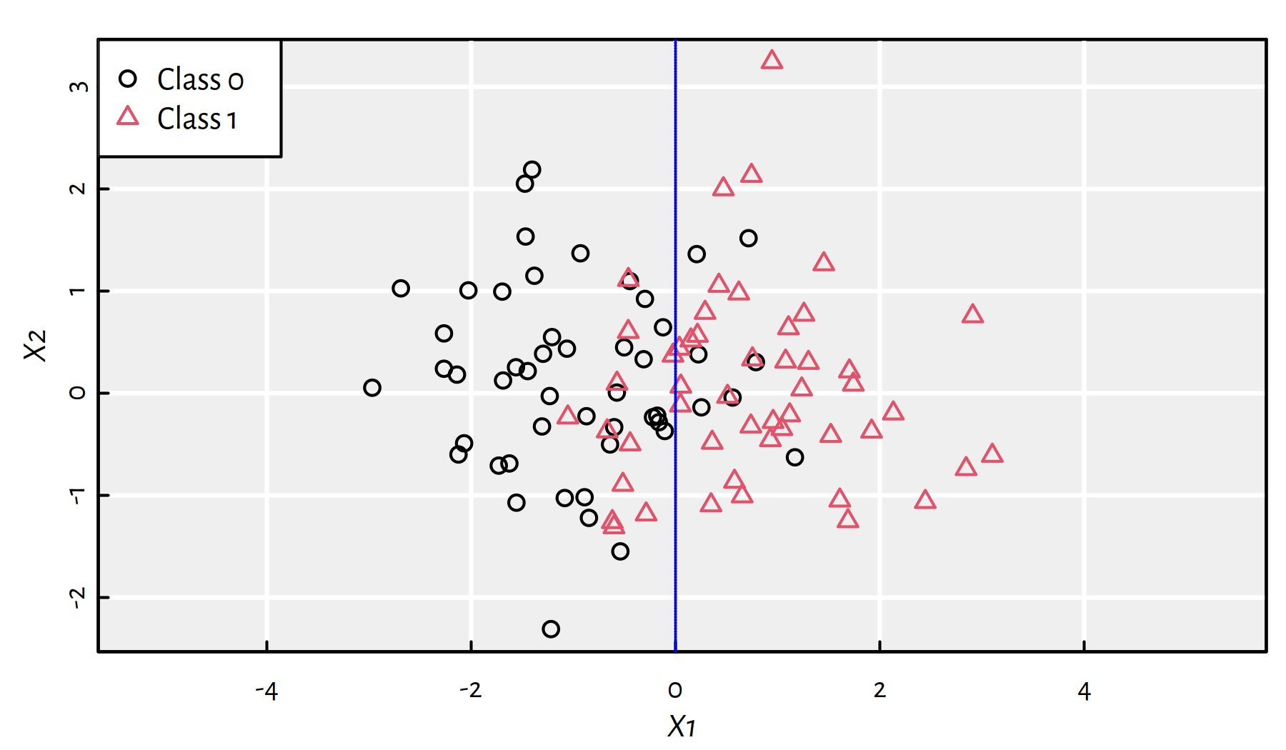
Figure 4.1: A synthetic 2D dataset with the true decision boundary at \(X_1=0\)
4.1.2 Data
For illustration, we’ll be considering the Wine Quality dataset (white wines only):
wines <- read.csv("datasets/winequality-all.csv",
    comment.char="#")
wines <- wines[wines$color == "white",]
(n <- nrow(wines)) # number of samples
## [1] 4898The input matrix \(\mathbf{X}\in\mathbb{R}^{n\times p}\) consists of the first 10 numeric variables:
X <- as.matrix(wines[,1:10])
dim(X)
## [1] 4898 10head(X, 2) # first two rows## fixed.acidity volatile.acidity citric.acid residual.sugar
## 1600 7.0 0.27 0.36 20.7
## 1601 6.3 0.30 0.34 1.6
## chlorides free.sulfur.dioxide total.sulfur.dioxide density pH
## 1600 0.045 45 170 1.001 3.0
## 1601 0.049 14 132 0.994 3.3
## sulphates
## 1600 0.45
## 1601 0.49The 11th variable measures the amount of alcohol (in %).
We will convert this dependent variable to a binary one:
- 0 == (
alcohol < 12) == lower-alcohol wines - 1 == (
alcohol >= 12) == higher-alcohol wines
# recall that TRUE == 1
Y <- factor(as.character(as.numeric(wines$alcohol >= 12)))
table(Y)
## Y
## 0 1
## 4085 81360/40% train-test split:
set.seed(123) # reproducibility matters
random_indices <- sample(n)
head(random_indices) # preview
## [1] 2463 2511 2227 526 4291 2986# first 60% of the indices (they are arranged randomly)
# will constitute the train sample:
train_indices <- random_indices[1:floor(n*0.6)]
X_train <- X[train_indices,]
Y_train <- Y[train_indices]
# the remaining indices (40%) go to the test sample:
X_test <- X[-train_indices,]
Y_test <- Y[-train_indices]Let’s also compute Z_train and Z_test, being the standardised versions of X_train
and X_test, respectively.
means <- apply(X_train, 2, mean) # column means
sds   <- apply(X_train, 2, sd)   # column standard deviations
Z_train <- t(apply(X_train, 1, function(r) (r-means)/sds))
Z_test  <- t(apply(X_test,  1, function(r) (r-means)/sds))
get_metrics <- function(Y_pred, Y_test)
{
C <- table(Y_pred, Y_test) # confusion matrix
stopifnot(dim(C) == c(2, 2))
c(Acc=(C[1,1]+C[2,2])/sum(C), # accuracy
Prec=C[2,2]/(C[2,2]+C[2,1]), # precision
Rec=C[2,2]/(C[2,2]+C[1,2]), # recall
F=C[2,2]/(C[2,2]+0.5*C[1,2]+0.5*C[2,1]), # F-measure
# Confusion matrix items:
TN=C[1,1], FN=C[1,2],
FP=C[2,1], TP=C[2,2]
) # return a named vector
}Let’s go back to the K-NN algorithm.
library("FNN")
Y_knn5 <- knn(X_train, X_test, Y_train, k=5)
Y_knn9 <- knn(X_train, X_test, Y_train, k=9)
Y_knn5s <- knn(Z_train, Z_test, Y_train, k=5)
Y_knn9s <- knn(Z_train, Z_test, Y_train, k=9)Recall the quality metrics we have obtained previously (as a point of reference):
cbind(
Knn5=get_metrics(Y_knn5, Y_test),
Knn9=get_metrics(Y_knn9, Y_test),
Knn5s=get_metrics(Y_knn5s, Y_test),
Knn9s=get_metrics(Y_knn9s, Y_test)
)## Knn5 Knn9 Knn5s Knn9s
## Acc 0.81735 0.81939 0.91429 0.91378
## Prec 0.38674 0.34959 0.82251 0.83636
## Rec 0.22082 0.13565 0.59937 0.58044
## F 0.28112 0.19545 0.69343 0.68529
## TN 1532.00000 1563.00000 1602.00000 1607.00000
## FN 247.00000 274.00000 127.00000 133.00000
## FP 111.00000 80.00000 41.00000 36.00000
## TP 70.00000 43.00000 190.00000 184.00000In this chapter we discuss the following simple and educational (yet practically useful) classification algorithms:
- decision trees,
- binary logistic regression.
4.2 Decision Trees
4.2.1 Introduction
Note that a K-NN classifier discussed in the previous chapter is model-free. The whole training set must be stored and referred to at all times.
Therefore, it doesn’t explain the data we have – we may use it solely for the purpose of prediction.
Perhaps one of the most interpretable (and hence human-friendly) models consist of decision rules of the form:
IF \(x_{i,j_1}\le v_1\) AND … AND \(x_{i,j_r}\le v_r\) THEN \(\hat{y}_i=1\).
These can be organised into a hierarchy for greater readability.
This idea inspired the notion of decision trees (Breiman et al. 1984).
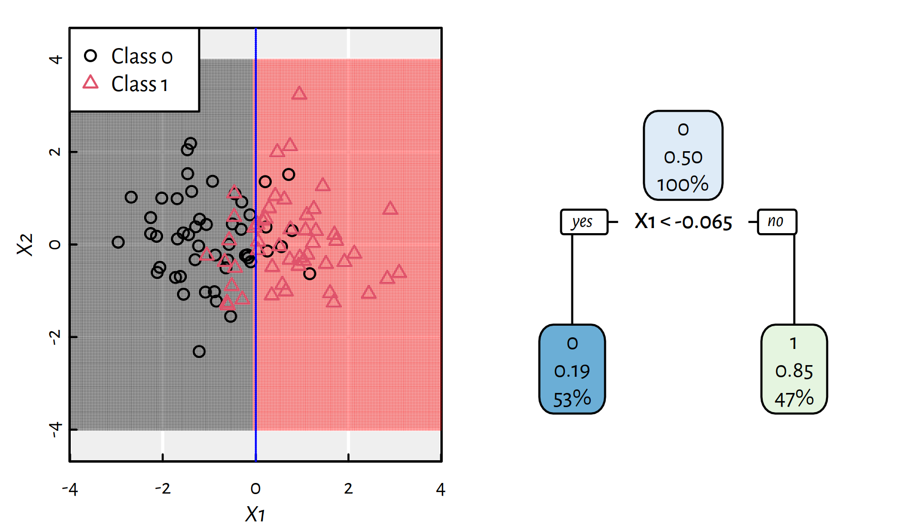
Figure 4.2: The simplest decision tree for the synthetic 2D dataset and the corresponding decision boundaries
Figure 4.2 depicts a very simple decision tree for the aforementioned synthetic dataset. There is only one decision boundary (based on \(X_1\)) that splits data into the “left” and “right” sides. Each tree node reports 3 pieces of information:
- dominating class (0 or 1)
- (relative) proportion of 1s represented in a node
- (absolute) proportion of all observations in a node
Figures 4.3 and 4.4 depict trees with more decision rules. Take a moment to contemplate how the corresponding decision boundaries changed with the introduction of new decision rules.
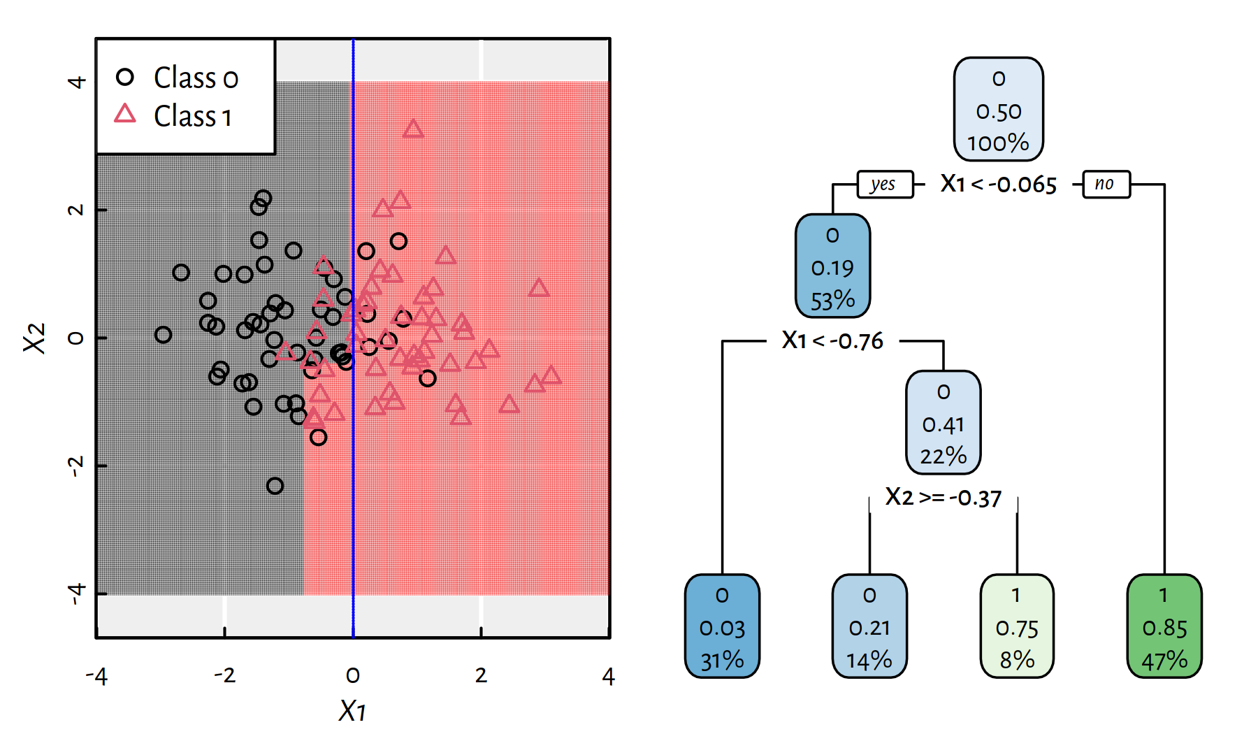
Figure 4.3: A more complicated decision tree for the synthetic 2D dataset and the corresponding decision boundaries
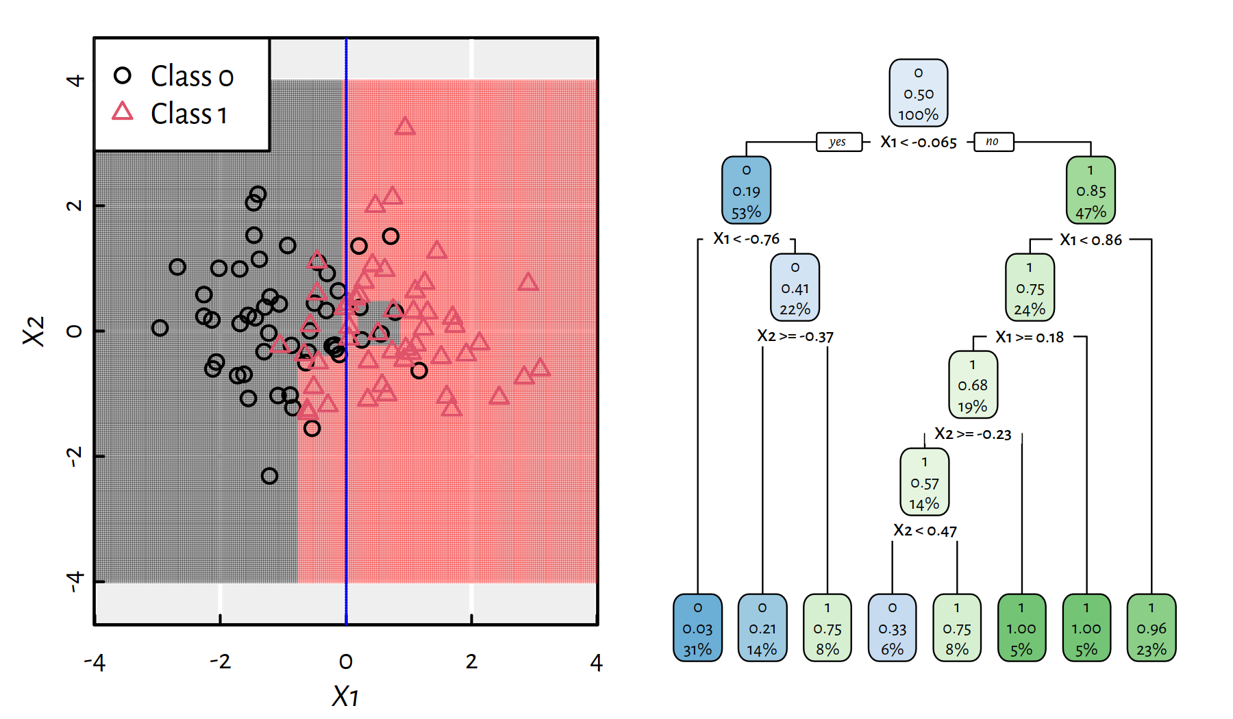
Figure 4.4: An even more complicated decision tree for the synthetic 2D dataset and the corresponding decision boundaries
4.2.2 Example in R
We will use the rpart() function from the rpart package
to build a classification tree.
library("rpart")
library("rpart.plot")
set.seed(123)rpart() uses a formula (~) interface, hence it will be easier
to feed it with data in a data.frame form.
XY_train <- cbind(as.data.frame(X_train), Y=Y_train)
XY_test <- cbind(as.data.frame(X_test), Y=Y_test)Fit and plot a decision tree, see Figure 4.5.
t1 <- rpart(Y~., data=XY_train, method="class")
rpart.plot(t1, tweak=1.1, fallen.leaves=FALSE, digits=3)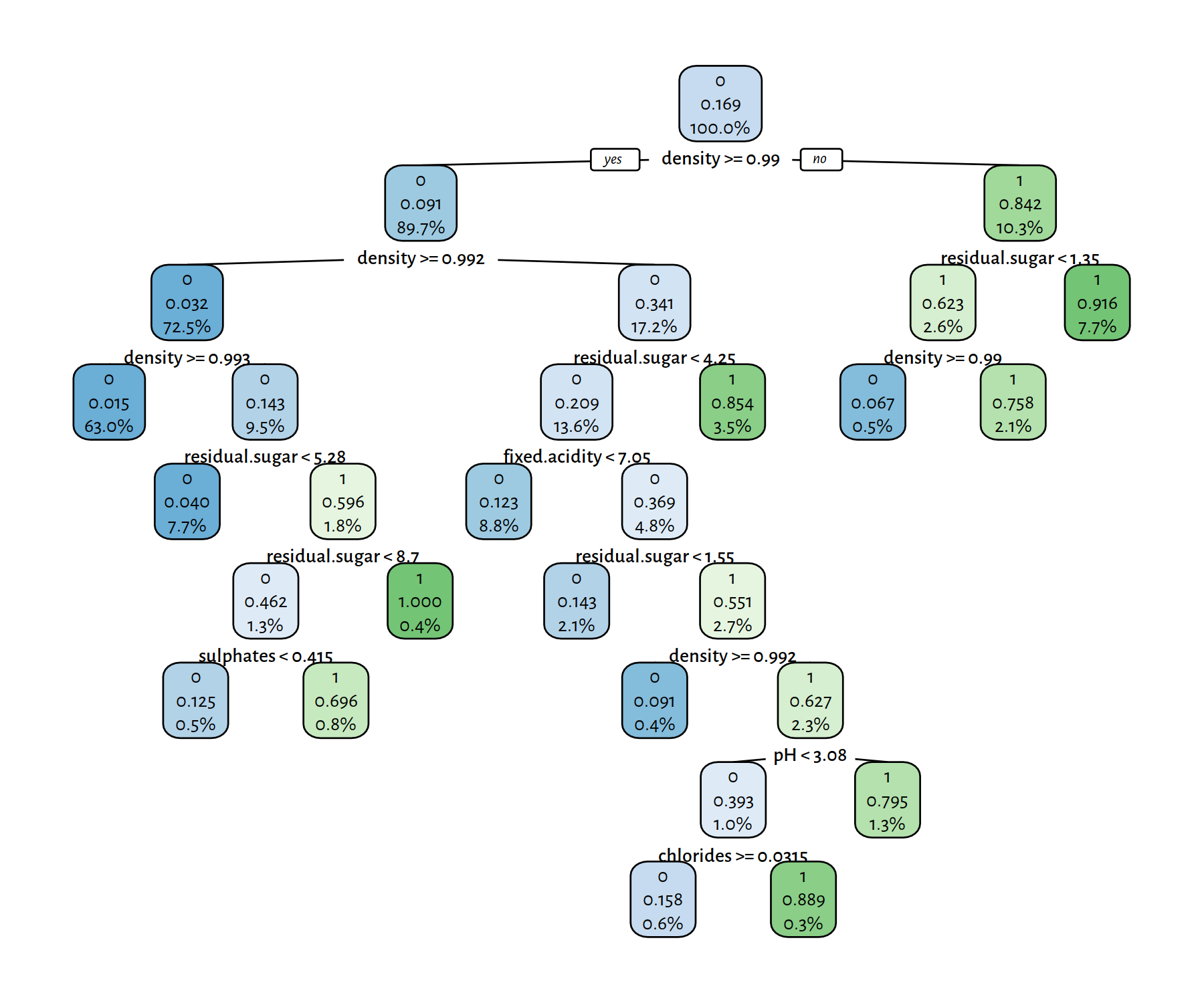
Figure 4.5: A decision tree for the wines dataset
We can build less or more complex trees by playing
with the cp parameter, see Figures 4.6
and 4.7.
# cp = complexity parameter, smaller → more complex tree
t2 <- rpart(Y~., data=XY_train, method="class", cp=0.1)
rpart.plot(t2, tweak=1.1, fallen.leaves=FALSE, digits=3)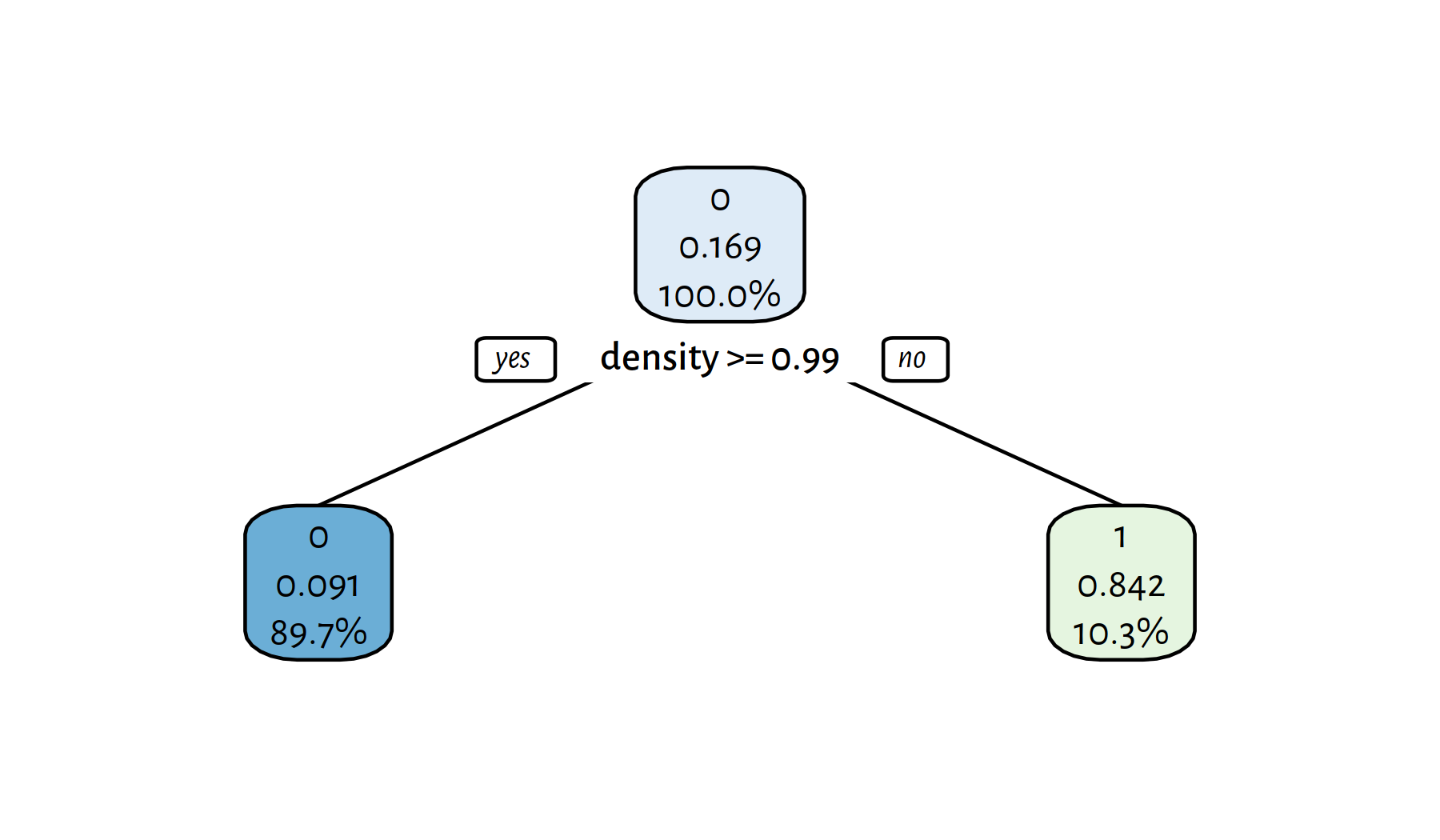
Figure 4.6: A (simpler) decision tree for the wines dataset
# cp = complexity parameter, smaller → more complex tree
t3 <- rpart(Y~., data=XY_train, method="class", cp=0.00001)
rpart.plot(t3, tweak=1.1, fallen.leaves=FALSE, digits=3)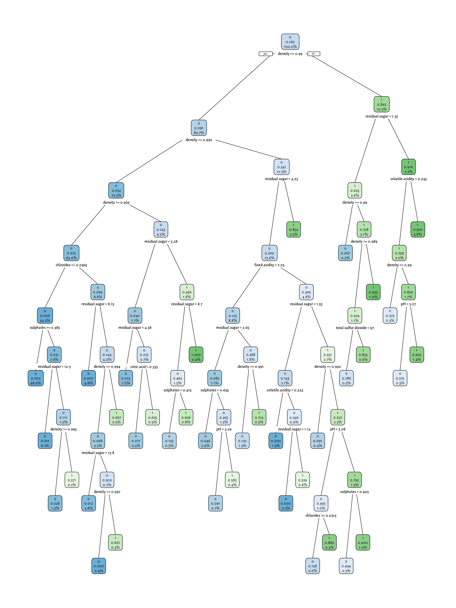
Figure 4.7: A (more complex) decision tree for the wines dataset
Trees with few decision rules actually are very nicely interpretable. On the other hand, plotting of the complex ones is just hopeless; we should treat them as “black boxes” instead.
Let’s make some predictions:
Y_pred <- predict(t1, XY_test, type="class")
get_metrics(Y_pred, Y_test)## Acc Prec Rec F TN FN
## 0.92857 0.80623 0.73502 0.76898 1587.00000 84.00000
## FP TP
## 56.00000 233.00000Y_pred <- predict(t2, XY_test, type="class")
get_metrics(Y_pred, Y_test)## Acc Prec Rec F TN FN
## 0.90255 0.83871 0.49211 0.62028 1613.00000 161.00000
## FP TP
## 30.00000 156.00000Y_pred <- predict(t3, XY_test, type="class")
get_metrics(Y_pred, Y_test)## Acc Prec Rec F TN FN
## 0.91837 0.73433 0.77603 0.75460 1554.00000 71.00000
## FP TP
## 89.00000 246.00000- Remark.
-
(*) Interestingly,
rpart()also provides us with information about the importance degrees of each independent variable.
t1$variable.importance/sum(t1$variable.importance)## density residual.sugar fixed.acidity
## 0.6562490 0.1984221 0.0305167
## chlorides pH volatile.acidity
## 0.0215008 0.0209678 0.0192880
## sulphates total.sulfur.dioxide citric.acid
## 0.0184293 0.0140482 0.0119201
## free.sulfur.dioxide
## 0.00865794.2.3 A Note on Decision Tree Learning
Learning an optimal decision tree is a computationally hard problem – we need some heuristics.
Examples:
- ID3 (Iterative Dichotomiser 3) (Quinlan 1986)
- C4.5 algorithm (Quinlan 1993)
- CART by Leo Breiman et al., (Breiman et al. 1984)
(**) Decision trees are most often constructed by a greedy, top-down recursive partitioning, see., e.g., (Therneau & Atkinson 2019).
4.3 Binary Logistic Regression
4.3.1 Motivation
Recall that for a regression task, we fitted a very simple family of models – the linear ones – by minimising the sum of squared residuals.
This approach was pretty effective.
(Very) theoretically, we could treat the class labels as numeric \(0\)s and \(1\)s and apply regression models in a binary classification task.
XY_train_r <- cbind(as.data.frame(X_train),
Y=as.numeric(Y_train)-1 # 0.0 or 1.0
)
XY_test_r <- cbind(as.data.frame(X_test),
Y=as.numeric(Y_test)-1 # 0.0 or 1.0
)
f_r <- lm(Y~density+residual.sugar+pH, data=XY_train_r)Y_pred_r <- predict(f_r, XY_test_r)
summary(Y_pred_r)## Min. 1st Qu. Median Mean 3rd Qu. Max.
## -3.0468 -0.0211 0.1192 0.1645 0.3491 0.8892The predicted outputs, \(\hat{Y}\), are arbitrary real numbers, but we can convert them to binary ones by checking if, e.g., \(\hat{Y}>0.5\).
Y_pred <- as.numeric(Y_pred_r>0.5)
round(get_metrics(Y_pred, XY_test_r$Y), 3)## Acc Prec Rec F TN FN FP TP
## 0.927 0.865 0.647 0.740 1611.000 112.000 32.000 205.000- Remark.
-
(*) The threshold \(T=0.5\) could even be treated as a free parameter we optimise for (w.r.t. different metrics over the validation sample), see Figure 4.8.
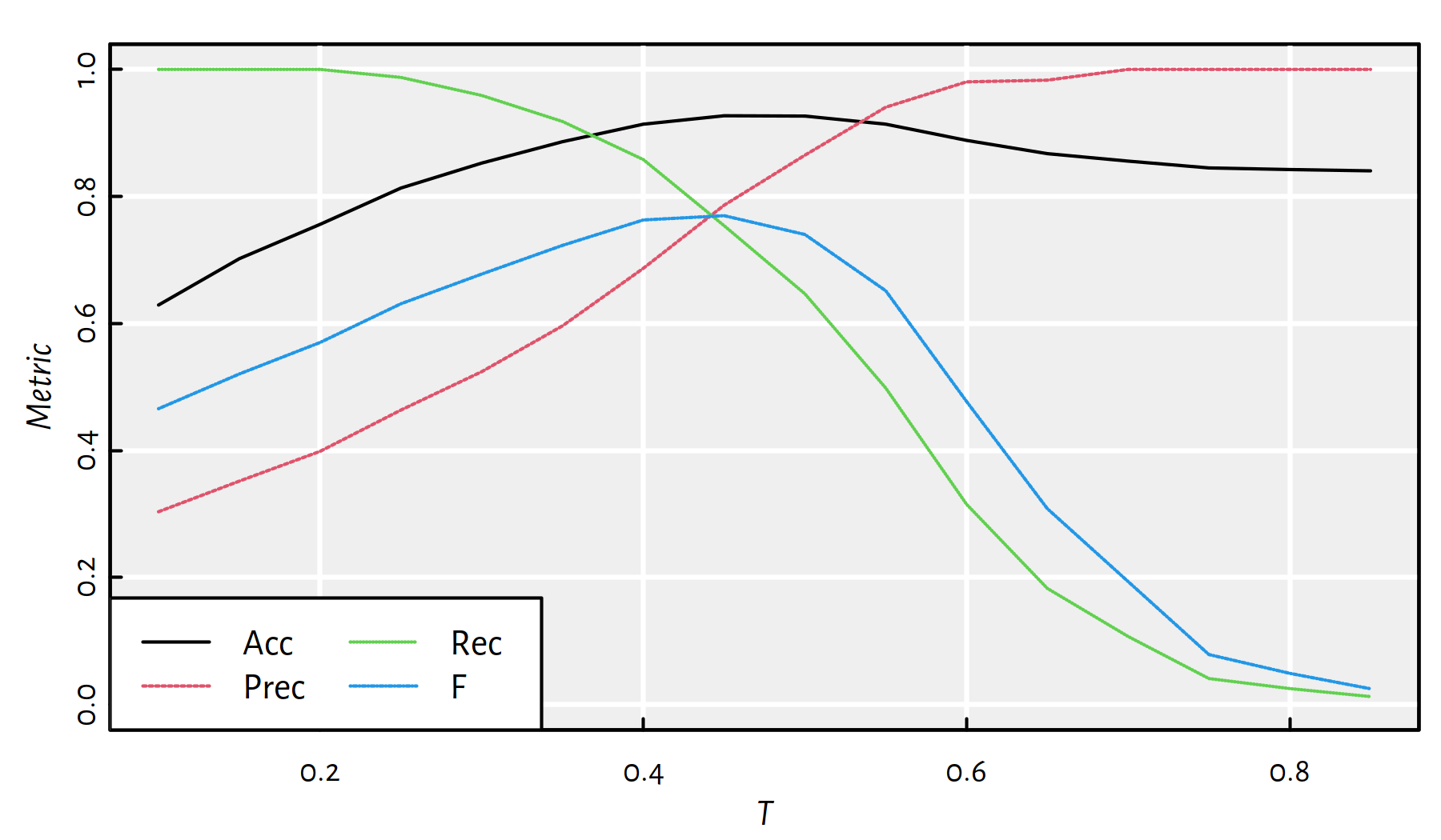
Figure 4.8: Quality metrics for a binary classifier “Classify X as 1 if \(f(X)>T\) and as 0 if \(f(X)\le T\)”
Despite we can, we shouldn’t use linear regression for classification. Treating class labels “0” and “1” as ordinary real numbers just doesn’t cut it – we intuitively feel that we are doing something ugly. Luckily, there is a better, more meaningful approach that still relies on a linear model, but has the right semantics.
4.3.2 Logistic Model
Inspired by this idea, we could try modelling the probability that a given point belongs to class \(1\).
This could also provide us with the confidence in our prediction.
Probability is a number in \([0,1]\), but the outputs of a linear model are arbitrary real numbers.
However, we could transform those real-valued outputs by means of some function \(\phi:\mathbb{R}\to[0,1]\) (preferably S-shaped == sigmoid), so as to get:
\[ \Pr(Y=1|\mathbf{X},\boldsymbol\beta)=\phi(\beta_0 + \beta_1 X_1 + \beta_2 X_2 + \dots + \beta_p X_p). \]
- Remark.
-
The above reads as “Probability that \(Y\) is from class 1 given \(\mathbf{X}\) and \(\boldsymbol\beta\)”.
A popular choice is the logistic sigmoid function, see Figure 4.9:
\[ \phi(t) = \frac{1}{1+e^{-t}} = \frac{e^t}{1+e^t}. \]
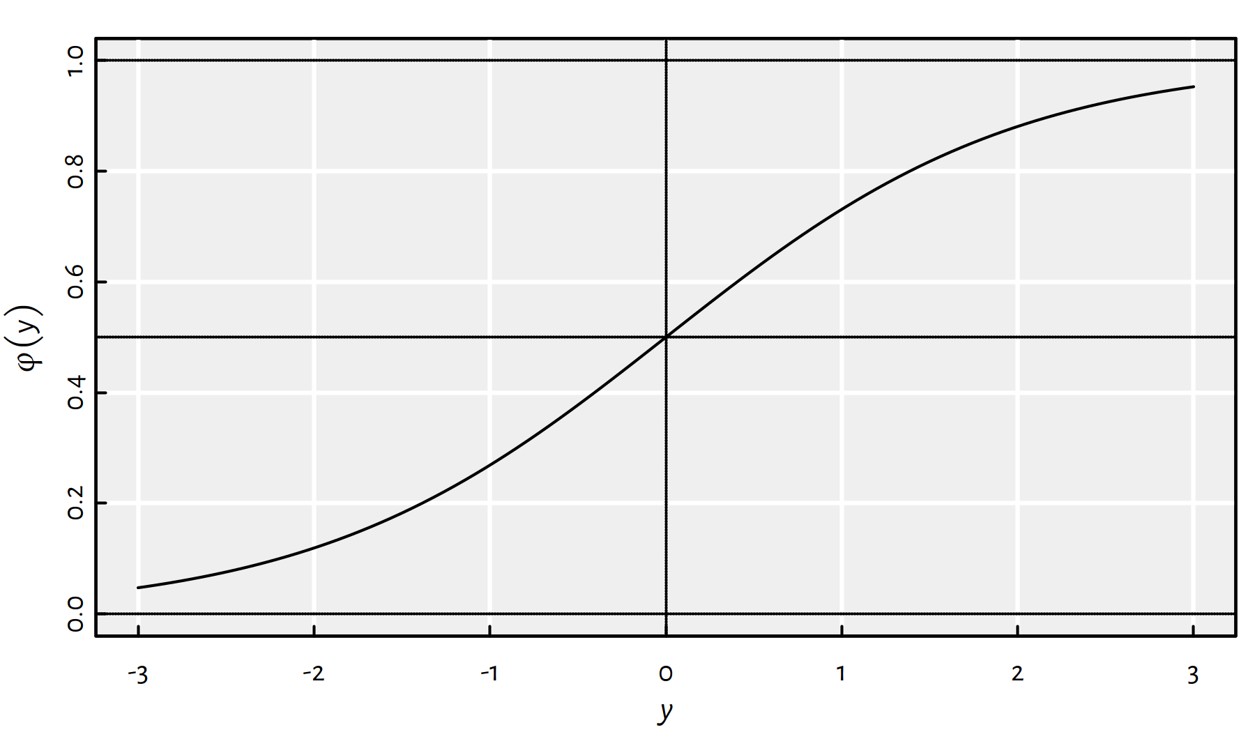
Figure 4.9: The logistic sigmoid function, \(\varphi\)
Hence our model becomes:
\[ Y=\frac{1}{1+e^{-(\beta_0 + \beta_1 X_1 + \beta_2 X_2 + \dots + \beta_p X_p)}} \]
It is an instance of a generalised linear model (glm) (there are of course many other possible generalisations).
4.3.3 Example in R
Let us first fit a simple (i.e., \(p=1\)) logistic regression model
using the density variable. The goodness-of-fit measure used in this
problem will be discussed a bit later.
(f <- glm(Y~density, data=XY_train, family=binomial("logit")))##
## Call: glm(formula = Y ~ density, family = binomial("logit"), data = XY_train)
##
## Coefficients:
## (Intercept) density
## 1173 -1184
##
## Degrees of Freedom: 2937 Total (i.e. Null); 2936 Residual
## Null Deviance: 2670
## Residual Deviance: 1420 AIC: 1420“logit” above denotes the inverse of the logistic sigmoid function. The fitted coefficients are equal to:
f$coefficients## (Intercept) density
## 1173.2 -1184.2Figure 4.10 depicts the obtained model, which can be written as: \[ \Pr(Y=1|x)=\displaystyle\frac{1}{1+e^{-\left( 1173.21-1184.21x \right)} } \] with \(x=\text{density}\).
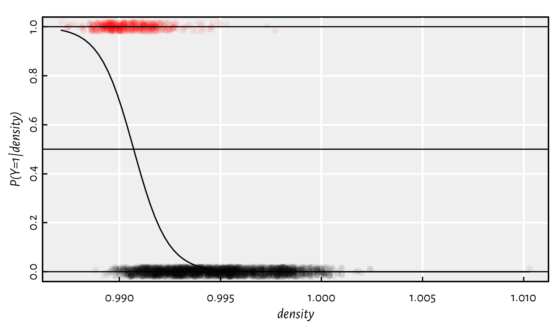
Figure 4.10: The probability that a given wine is a high-alcohol one given its density; black and red points denote the actual observed data points from the class 0 and 1, respectively
Some predicted probabilities:
round(head(predict(f, XY_test, type="response"), 12), 2)## 1602 1605 1607 1608 1609 1613 1614 1615 1621 1622 1623 1627
## 0.01 0.01 0.00 0.02 0.03 0.36 0.00 0.31 0.36 0.06 0.03 0.00We classify \(Y\) as 1 if the corresponding membership probability is greater than \(0.5\).
Y_pred <- as.numeric(predict(f, XY_test, type="response")>0.5)
get_metrics(Y_pred, Y_test)## Acc Prec Rec F TN FN
## 0.89796 0.72763 0.58991 0.65157 1573.00000 130.00000
## FP TP
## 70.00000 187.00000And now a fit based on some other input variables:
(f <- glm(Y~density+residual.sugar+total.sulfur.dioxide,
data=XY_train, family=binomial("logit")))##
## Call: glm(formula = Y ~ density + residual.sugar + total.sulfur.dioxide,
## family = binomial("logit"), data = XY_train)
##
## Coefficients:
## (Intercept) density residual.sugar
## 2.50e+03 -2.53e+03 8.58e-01
## total.sulfur.dioxide
## 9.74e-03
##
## Degrees of Freedom: 2937 Total (i.e. Null); 2934 Residual
## Null Deviance: 2670
## Residual Deviance: 920 AIC: 928Y_pred <- as.numeric(predict(f, XY_test, type="response")>0.5)
get_metrics(Y_pred, Y_test)## Acc Prec Rec F TN FN
## 0.93214 0.82394 0.73817 0.77870 1593.00000 83.00000
## FP TP
## 50.00000 234.00000Try fitting different models based on other sets of features.
4.3.4 Loss Function: Cross-entropy
The fitting of the model can be written as an optimisation task:
\[ \min_{\beta_0, \beta_1,\dots, \beta_p\in\mathbb{R}} \frac{1}{n} \sum_{i=1}^n \epsilon\left(\hat{y}_i, y_i \right) \]
where \(\epsilon(\hat{y}_i, y_i)\) denotes the penalty that measures the “difference” between the true \(y_i\) and its predicted version \(\hat{y}_i=\Pr(Y=1|\mathbf{x}_{i,\cdot},\boldsymbol\beta)\).
In the ordinary regression, we used the squared residual \(\epsilon(\hat{y}_i, y_i) = (\hat{y}_i-y_i)^2\). In logistic regression (the kind of a classifier we are interested in right now), we use the cross-entropy (a.k.a. log-loss, binary cross-entropy),
\[ \epsilon(\hat{y}_i,y_i) = - \left(y_i \log \hat{y}_i + (1-y_i) \log(1-\hat{y}_i)\right) \]
The corresponding loss function has not only many nice statistical properties (** related to maximum likelihood estimation etc.) but also an intuitive interpretation.
Note that the predicted \(\hat{y}_i\) is in \((0,1)\) and the true \(y_i\) equals to either 0 or 1. Recall also that \(\log t\in(-\infty, 0)\) for \(t\in (0,1)\). Therefore, the formula for \(\epsilon(\hat{y}_i,y_i)\) has a very intuitive behaviour:
if true \(y_i=1\), then the penalty becomes \(\epsilon(\hat{y}_i, 1) = -\log(\hat{y}_i)\)
- \(\hat{y}_i\) is the probability that the classified input is indeed from class \(1\)
- we’d be happy if the classifier outputted \(\hat{y}_i\simeq 1\) in this case; this is not penalised as \(-\log(t)\to 0\) as \(t\to 1\)
- however, if the classifier is totally wrong, i.e., it thinks that \(\hat{y}_i\simeq 0\), then the penalty will be very high, as \(-\log(t)\to+\infty\) as \(t\to 0\)
if true \(y_i=0\), then the penalty becomes \(\epsilon(\hat{y}_i, 0) = -\log(1-\hat{y}_i)\)
- \(1-\hat{y}_i\) is the predicted probability that the input is from class \(0\)
- we penalise heavily the case where \(1-\hat{y}_i\) is small (we’d be happy if the classifier was sure that \(1-\hat{y}_i\simeq 1\), because this is the ground-truth)
(*) Having said that, let’s expand the above formulae. The task of minimising cross-entropy in the binary logistic regression can be written as \(\min_{\boldsymbol\beta\in\mathbb{R}^{p+1}} E(\boldsymbol\beta)\) with:
\[ E(\boldsymbol\beta)= -\frac{1}{n} \sum_{i=1}^n y_i \log \Pr(Y=1|\mathbf{x}_{i,\cdot},\boldsymbol\beta) + (1-y_i) \log(1-\Pr(Y=1|\mathbf{x}_{i,\cdot},\boldsymbol\beta)) \]
Taking into account that:
\[ \Pr(Y=1|\mathbf{x}_{i,\cdot},\boldsymbol\beta)= \frac{1}{1+e^{-(\beta_0 + \beta_1 x_{i,1}+\dots+\beta_p x_{i,p})}}, \]
we get:
\[ E(\boldsymbol\beta)= -\frac{1}{n} \sum_{i=1}^n \left( \begin{array}{r} y_i \log \displaystyle\frac{1}{1+e^{-(\beta_0 + \beta_1 x_{i,1}+\dots+\beta_p x_{i,p})}}\\ + (1-y_i) \log \displaystyle\frac{e^{-(\beta_0 + \beta_1 x_{i,1}+\dots+\beta_p x_{i,p})}}{1+e^{-(\beta_0 + \beta_1 x_{i,1}+\dots+\beta_p x_{i,p})}} \end{array} \right). \]
Logarithms are really practitioner-friendly functions, it holds:
- \(\log 1=0\),
- \(\log e=1\) (where \(e \simeq 2.71828\) is the Euler constant; note that by writing \(\log\) we mean the natural a.k.a. base-\(e\) logarithm),
- \(\log xy = \log x + \log y\),
- \(\log x^p = p\log x\) (this is \(\log (x^p)\), not \((\log x)^p\)).
These facts imply, amongst others that:
- \(\log e^x = x \log e = x\),
- \(\log \frac{x}{y} = \log x y^{-1} = \log x+\log y^{-1} = \log x - \log y\) (of course for \(y\neq 0\)),
- \(\log \frac{1}{y} = -\log y\)
and so forth. Therefore, based on the fact that \(1/(1+e^{-x})=e^x/(1+e^x)\), the above optimisation problem can be rewritten as:
\[ E(\boldsymbol\beta)= \frac{1}{n} \sum_{i=1}^n \left( \begin{array}{r} y_i \log \left(1+e^{-(\beta_0 + \beta_1 x_{i,1}+\dots+\beta_p x_{i,p})}\right)\\ + (1-y_i) \log \left(1+e^{+(\beta_0 + \beta_1 x_{i,1}+\dots+\beta_p x_{i,p})}\right) \end{array} \right) \]
or, if someone prefers:
\[ E(\boldsymbol\beta)= \frac{1}{n} \sum_{i=1}^n \left( (1-y_i)\left(\beta_0 + \beta_1 x_{i,1}+\dots+\beta_p x_{i,p}\right) +\log \left(1+e^{-(\beta_0 + \beta_1 x_{i,1}+\dots+\beta_p x_{i,p})}\right) \right). \]
It turns out that there is no analytical formula
for the optimal set of parameters (\(\beta_0,\beta_1,\dots,\beta_p\)
minimising the log-loss).
In the chapter on optimisation, we shall see that
the solution to the logistic regression can be solved numerically
by means of quite simple iterative algorithms.
The two expanded formulae have lost the appealing interpretation
of the original one, however, it’s more numerically well-behaving,
see, e.g., the log1p() function in base R or, even better,
fermi_dirac_0() in the gsl package.
4.4 Exercises in R
4.4.1 EdStats – Preparing Data
In this exercise, we will prepare the EdStats dataset
for further analysis.
The file edstats_2019.csv provides us with many
country-level Education Statistics extracted from the World Bank’s Databank,
see https://databank.worldbank.org/.
Databank aggregates information from such sources as
the UNESCO Institute for Statistics,
OECD Programme for International Student Assessment (PISA)
etc. The official description reads:
“The World Bank EdStats Query holds around 2,500 internationally comparable education indicators for access, progression, completion, literacy, teachers, population, and expenditures. The indicators cover the education cycle from pre-primary to tertiary education. The query also holds learning outcome data from international learning assessments (PISA, TIMSS, etc.), equity data from household surveys, and projection data to 2050.”
edstats_2019.csv was compiled on 24 April 2020 and lists
indicators reported between 2010 and 2019.
First, let’s load the dataset:
edstats_2019 <- read.csv("datasets/edstats_2019.csv",
comment.char="#")
head(edstats_2019)## CountryName CountryCode
## 1 Afghanistan AFG
## 2 Afghanistan AFG
## 3 Afghanistan AFG
## 4 Afghanistan AFG
## 5 Afghanistan AFG
## 6 Afghanistan AFG
## Series
## 1 Government expenditure on education as % of GDP (%)
## 2 Gross enrolment ratio, primary, female (%)
## 3 Net enrolment rate, primary, female (%)
## 4 Primary completion rate, both sexes (%)
## 5 PISA: Mean performance on the mathematics scale
## 6 PISA: Mean performance on the mathematics scale. Female
## Code Y2010 Y2011 Y2012 Y2013 Y2014 Y2015
## 1 SE.XPD.TOTL.GD.ZS 3.4794 3.462 2.6042 3.4545 3.6952 3.2558
## 2 SE.PRM.ENRR.FE 80.6355 80.937 86.3288 85.9021 86.7296 83.5044
## 3 SE.PRM.NENR.FE NA NA NA NA NA NA
## 4 SE.PRM.CMPT.ZS NA NA NA NA NA NA
## 5 LO.PISA.MAT NA NA NA NA NA NA
## 6 LO.PISA.MAT.FE NA NA NA NA NA NA
## Y2016 Y2017 Y2018 Y2019
## 1 4.2284 4.0589 NA NA
## 2 82.5584 82.0803 82.850 NA
## 3 NA NA NA NA
## 4 79.9346 84.4150 85.625 NA
## 5 NA NA NA NA
## 6 NA NA NA NAThis data frame is in a “long” format, where each indicator for each country is given in its own row. Note that some indicators are not surveyed/updated every year.
Convert edstats_2019 to a “wide” format (one row per country,
each indicator in its own column) based on the most recent observed indicators.
Click here for a solution.
First we need a function that returns the last non-missing value in a
given numeric vector.
To recall, na.omit(), removes all missing values and tail() can be
used to access the last observation easily. Unfortunately, if the vector
is consists of missing values only, the removal of NAs leads
to an empty sequence. However, the trick we can use is that
by extracting the first element from an empty vector by using
[...], we get a NA.
last_non_na <- function(x) tail(na.omit(x), 1)[1]
last_non_na(c(1, 2, NA, 3,NA,NA)) # example 1## [1] 3last_non_na(c(NA,NA,NA,NA,NA,NA)) # example 2## [1] NALet’s extract the most recent indicator from each row in edstats_2019.
values <- apply(edstats_2019[-(1:4)], 1, last_non_na)
head(values)## [1] 4.0589 82.8503 NA 85.6253 NA NANow, we shall create a data frame with 3 columns: name of the country, indicator code, indicator value. Let’s order it with respect to the first two columns.
edstats_2019 <- edstats_2019[c("CountryName", "Code")]
# add a new column at the righthand end:
edstats_2019["Value"] <- values
edstats_2019 <- edstats_2019[
order(edstats_2019$CountryName, edstats_2019$Code), ]
head(edstats_2019)## CountryName Code Value
## 59 Afghanistan HD.HCI.AMRT 0.7797
## 57 Afghanistan HD.HCI.AMRT.FE 0.8018
## 58 Afghanistan HD.HCI.AMRT.MA 0.7597
## 53 Afghanistan HD.HCI.EYRS 8.5800
## 51 Afghanistan HD.HCI.EYRS.FE 6.7300
## 52 Afghanistan HD.HCI.EYRS.MA 9.2100To convert the data frame to a “wide” format, many readers would choose
the pivot_wider() function from the tidyr package
(amongst others).
library("tidyr")
edstats <- as.data.frame(
pivot_wider(edstats_2019, names_from="Code", values_from="Value")
)
edstats[1, 1:7]## CountryName HD.HCI.AMRT HD.HCI.AMRT.FE HD.HCI.AMRT.MA HD.HCI.EYRS
## 1 Afghanistan 0.7797 0.8018 0.7597 8.58
## HD.HCI.EYRS.FE HD.HCI.EYRS.MA
## 1 6.73 9.21On a side note (*), the above solution is of course perfectly fine and we can now live long and prosper. Nevertheless, we are here to learn new skills, so let’s note that it has the drawback that it required us to search for the answer on the internet (and go through many “answers” that actually don’t work). If we are not converting between the long and the wide formats on a daily basis, this might not be worth the hassle (moreover, there’s no guarantee that this function will work the same way in the future, that the package we relied on will provide the same API etc.).
Instead, by relaying on a bit deeper knowledge of R programming (which we already have, see Appendices A-D of our book), we could implement the relevant procedure manually. The downside is that this requires us to get out of our comfort zone and… think.
First, let’s generate the list of all countries and indicators:
countries <- unique(edstats_2019$CountryName)
head(countries)## [1] "Afghanistan" "Albania" "Algeria" "American Samoa"
## [5] "Andorra" "Angola"indicators <- unique(edstats_2019$Code)
head(indicators)## [1] "HD.HCI.AMRT" "HD.HCI.AMRT.FE" "HD.HCI.AMRT.MA" "HD.HCI.EYRS"
## [5] "HD.HCI.EYRS.FE" "HD.HCI.EYRS.MA"Second, note that edstats_2019 gives all the possible combinations (pairs)
of the indexes and countries:
nrow(edstats_2019) # number of rows in edstats_2019## [1] 23852length(countries)*length(indicators) # number of pairs## [1] 23852Looking at the numbers in the Value column of edstats_2019,
this will exactly provide us with our desired “wide” data matrix,
if we read it in a rowwise manner. Hence, we can use
matrix(..., byrow=TRUE) to generate it:
# edstats_2019 is already sorted w.r.t. CountryName and Code
edstats2 <- cbind(
CountryName=countries, # first column
as.data.frame(
matrix(edstats_2019$Value,
byrow=TRUE,
ncol=length(indicators),
dimnames=list(NULL, indicators)
)))
identical(edstats, edstats2)## [1] TRUEExport edstats to a CSV file.
Click here for a solution.
This can be done as follows:
write.csv(edstats, "edstats_2019_wide.csv", row.names=FALSE)We didn’t export the row names, because they’re useless in our case.
Explore edstats_meta.csv to understand the meaning of the
EdStats indicators.
Click here for a solution.
First, let’s load the dataset:
meta <- read.csv("datasets/edstats_meta.csv")
names(meta) # column names## [1] "Code" "Series" "Definition" "Source" "Topic"The Series column deciphers each indicator’s meaning.
For instance, LO.PISA.MAT gives:
meta[meta$Code=="LO.PISA.MAT", "Series"]## [1] "PISA: Mean performance on the mathematics scale"To get more information, we can take a look at the Definition
column:
meta[meta$Code=="LO.PISA.MAT", "Definition"]which reads: Average score of 15-year-old students on the PISA mathematics scale. The metric for the overall mathematics scale is based on a mean for OECD countries of 500 points and a standard deviation of 100 points. Data reflects country performance in the stated year according to PISA reports, but may not be comparable across years or countries. Consult the PISA website for more detailed information: http://www.oecd.org/pisa/.
4.4.2 EdStats – Where Girls Are Better at Maths Than Boys?
In this task we will consider the “wide” version of the EdStats dataset:
edstats <- read.csv("datasets/edstats_2019_wide.csv",
comment.char="#")
edstats[1, 1:6]## CountryName HD.HCI.AMRT HD.HCI.AMRT.FE HD.HCI.AMRT.MA HD.HCI.EYRS
## 1 Afghanistan 0.7797 0.8018 0.7597 8.58
## HD.HCI.EYRS.FE
## 1 6.73meta <- read.csv("datasets/edstats_meta.csv")This dataset is small, moreover, we’ll be more interested in the description (understanding) of data, not prediction of the response variable to unobserved samples. Note that we have the population of the World countries at hand here (new countries do not arise on a daily basis). Therefore, a train-test split won’t be performed.
Add a 0/1 factor-type variable girls_rule_maths that is equal to 1
if and only if a country’s average score of 15-year-old female students on the PISA
mathematics scale is greater than the corresponding indicator for the male ones.
Click here for a solution.
Recall that a conversion of a logical value to a number
yields 1 for TRUE and 0 for FALSE. Hence:
edstats$girls_rule_maths <-
factor(as.numeric(
edstats$LO.PISA.MAT.FE>edstats$LO.PISA.MAT.MA
))
head(edstats$girls_rule_maths, 10)## [1] <NA> 1 1 <NA> <NA> <NA> <NA> <NA> 0 <NA>
## Levels: 0 1Unfortunately, there are many missing values in the dataset. More precisely:
sum(is.na(edstats$girls_rule_maths)) # count## [1] 187mean(is.na(edstats$girls_rule_maths)) # proportion## [1] 0.69776Countries such as Egypt, India, Iran or Venezuela are not amongst the 79 members of the Programme for International Student Assessment. Thus, we’ll have to deal with the data we have.
The percentage of counties where “girls rule” is equal to:
mean(edstats$girls_rule_maths==1, na.rm=TRUE)## [1] 0.33333Here is the list of those counties:
as.character(na.omit(
edstats[edstats$girls_rule_maths==1, "CountryName"]
))## [1] "Albania" "Algeria"
## [3] "Brunei Darussalam" "Bulgaria"
## [5] "Cyprus" "Dominican Republic"
## [7] "Finland" "Georgia"
## [9] "Hong Kong SAR, China" "Iceland"
## [11] "Indonesia" "Israel"
## [13] "Jordan" "Lithuania"
## [15] "Malaysia" "Malta"
## [17] "Moldova" "North Macedonia"
## [19] "Norway" "Philippines"
## [21] "Qatar" "Saudi Arabia"
## [23] "Sweden" "Thailand"
## [25] "Trinidad and Tobago" "United Arab Emirates"
## [27] "Vietnam"Learn a decision tree that distinguishes between the countries where girls are better at maths than boys and assess the quality of this classifier.
Click here for a solution.
Let’s first create a subset of edstats that doesn’t include
the country names as well as the boys’ and girls’ math scores.
edstats_subset <- edstats[!(names(edstats) %in%
c("CountryName", "LO.PISA.MAT.FE", "LO.PISA.MAT.MA"))]Fitting and plotting (see Figure 4.11) of the tree can be performed as follows:
library("rpart")
library("rpart.plot")
tree <- rpart(girls_rule_maths~., data=edstats_subset,
method="class", model=TRUE)
rpart.plot(tree)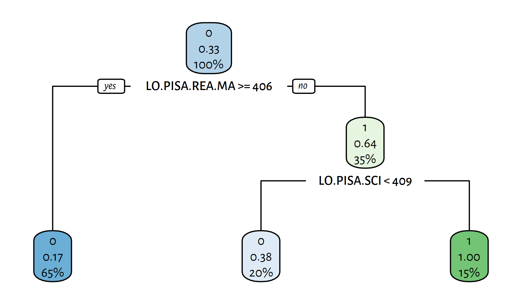
Figure 4.11: A decision tree explaining the girls_rule_maths variable
The variables included in the model are:
Note that the decision rules are well-interpretable, we can make a whole story around it. Whether or not it is actually true – is a different… story.
To compute the basic classifier performance scores,
let’s recall the get_metrics() function:
get_metrics <- function(Y_pred, Y_test)
{
    C <- table(Y_pred, Y_test) # confusion matrix
    stopifnot(dim(C) == c(2, 2))
    c(Acc=(C[1,1]+C[2,2])/sum(C), # accuracy
      Prec=C[2,2]/(C[2,2]+C[2,1]), # precision
      Rec=C[2,2]/(C[2,2]+C[1,2]), # recall
      F=C[2,2]/(C[2,2]+0.5*C[1,2]+0.5*C[2,1]), # F-measure
      # Confusion matrix items:
      TN=C[1,1], FN=C[1,2],
      FP=C[2,1], TP=C[2,2]
    ) # return a named vector
}Now we can judge the tree’s character:
Y_pred <- predict(tree, edstats_subset, type="class")
get_metrics(Y_pred, edstats_subset$girls_rule_maths)## Acc Prec Rec F TN FN FP TP
## 0.81481 1.00000 0.44444 0.61538 54.00000 15.00000 0.00000 12.00000Learn a decision tree that this time doesn’t rely on any of the PISA indicators.
Click here for a solution.
Let’s remove the unwanted variables:
edstats_subset <- edstats[!(names(edstats) %in%
c("LO.PISA.MAT", "LO.PISA.MAT.FE", "LO.PISA.MAT.MA",
"LO.PISA.REA", "LO.PISA.REA.FE", "LO.PISA.REA.MA",
"LO.PISA.SCI", "LO.PISA.SCI.FE", "LO.PISA.SCI.MA",
"CountryName"))]On a side note, this could be done more easily by calling, e.g.,
stri_startswith_fixed(names(edstats), "LO.PISA") from the stringi package.
Fitting and plotting (see Figure 4.12) of the tree:
tree <- rpart(girls_rule_maths~., data=edstats_subset,
method="class", model=TRUE)
rpart.plot(tree)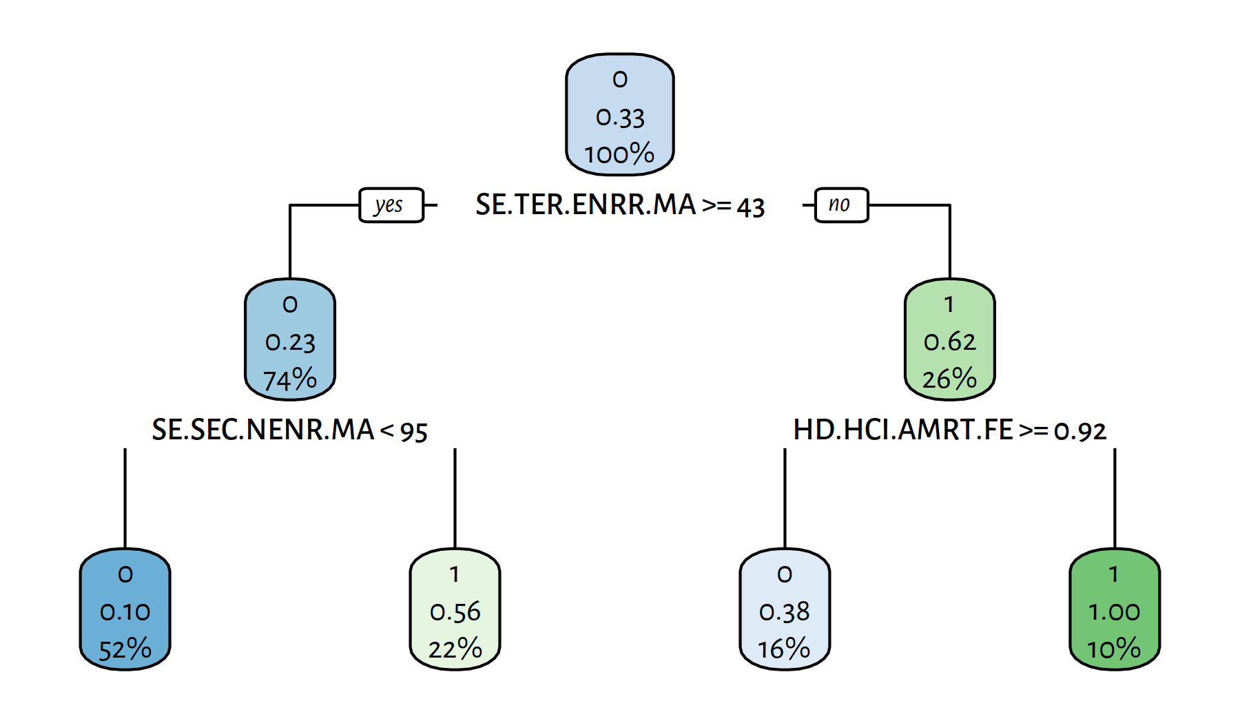
Figure 4.12: Another decision tree explaining the girls_rule_maths variable
Performance metrics:
Y_pred <- predict(tree, edstats, type="class")
get_metrics(Y_pred, edstats_subset$girls_rule_maths)## Acc Prec Rec F TN FN FP TP
## 0.79012 0.69231 0.66667 0.67925 46.00000 9.00000 8.00000 18.00000It’s interesting to note that some of the goodness-of-fit measures are actually higher now.
The variables included in the model are:
4.4.3 EdStats and World Factbook – Joining Forces
In the course of our data science journey, we have considered two datasets dealing with country-level indicators: the World Factbook and World Bank’s EdStats.
factbook <- read.csv("datasets/world_factbook_2020.csv",
comment.char="#")
edstats <- read.csv("datasets/edstats_2019_wide.csv",
comment.char="#")Let’s combine the information they provide and see if we come up with a better model of where girls’ math scores are higher.
Some country names in one dataset don’t match those in the other one, for instance: Czech Republic vs. Czechia, Myanmar vs. Burma, etc. Resolve these conflicts as best you can.
Click here for a solution.
To get a list of the mismatched country names, we can call either:
factbook$country[!(factbook$country %in% edstats$CountryName)]or:
edstats$CountryName[!(edstats$CountryName %in% factbook$country)]Unfortunately, the data need to be cleaned manually – it’s a tedious task. The following consists of what we hope are the best matches between the two datasets (yet, the list is not perfect; in particular, the Republic of North Macedonia is completely missing in one of the datasets):
from_to <- matrix(ncol=2, byrow=TRUE, c(
# FROM (edstats) # TO (factbook)
"Brunei Darussalam" , "Brunei" ,
"Congo, Dem. Rep." , "Congo, Democratic Republic of the" ,
"Congo, Rep." , "Congo, Republic of the" ,
"Czech Republic" , "Czechia" ,
"Egypt, Arab Rep." , "Egypt" ,
"Hong Kong SAR, China" , "Hong Kong" ,
"Iran, Islamic Rep." , "Iran" ,
"Korea, Dem. People’s Rep." , "Korea, North" ,
"Korea, Rep." , "Korea, South" ,
"Kyrgyz Republic" , "Kyrgyzstan" ,
"Lao PDR" , "Laos" ,
"Macao SAR, China" , "Macau" ,
"Micronesia, Fed. Sts." , "Micronesia, Federated States of" ,
"Myanmar" , "Burma" ,
"Russian Federation" , "Russia" ,
"Slovak Republic" , "Slovakia" ,
"St. Kitts and Nevis" , "Saint Kitts and Nevis" ,
"St. Lucia" , "Saint Lucia" ,
"St. Martin (French part)" , "Saint Martin" ,
"St. Vincent and the Grenadines", "Saint Vincent and the Grenadines" ,
"Syrian Arab Republic" , "Syria" ,
"Venezuela, RB" , "Venezuela" ,
"Virgin Islands (U.S.)" , "Virgin Islands" ,
"Yemen, Rep." , "Yemen"
))Conversion of the names:
for (i in 1:nrow(from_to)) {
edstats$CountryName[edstats$CountryName==from_to[i,1]] <- from_to[i,2]
}On a side note (*), this could be done with a single call to
a function in the stringi package:
library("stringi")
edstats$CountryName <- stri_replace_all_fixed(edstats$CountryName,
from_to[,1], from_to[,2], vectorize_all=FALSE)Merge (join) the two datasets based on the country names.
Click here for a solution.
This can be done by means of the merge() function.
edbook <- merge(edstats, factbook, by.x="CountryName", by.y="country")
ncol(edbook) # how many columns we have now## [1] 157Learn a decision tree that distinguishes between the countries where girls are better at maths than boys and assess the quality of this classifier.
Click here for a solution.
We proceed as in one of the previous exercises:
edbook$girls_rule_maths <-
factor(as.numeric(
edbook$LO.PISA.MAT.FE>edbook$LO.PISA.MAT.MA
))
edbook_subset <- edbook[!(names(edbook) %in%
c("CountryName", "LO.PISA.MAT.FE", "LO.PISA.MAT.MA"))]Fitting and plotting (see Figure 4.13):
library("rpart")
library("rpart.plot")
tree <- rpart(girls_rule_maths~., data=edbook_subset,
method="class", model=TRUE)
rpart.plot(tree)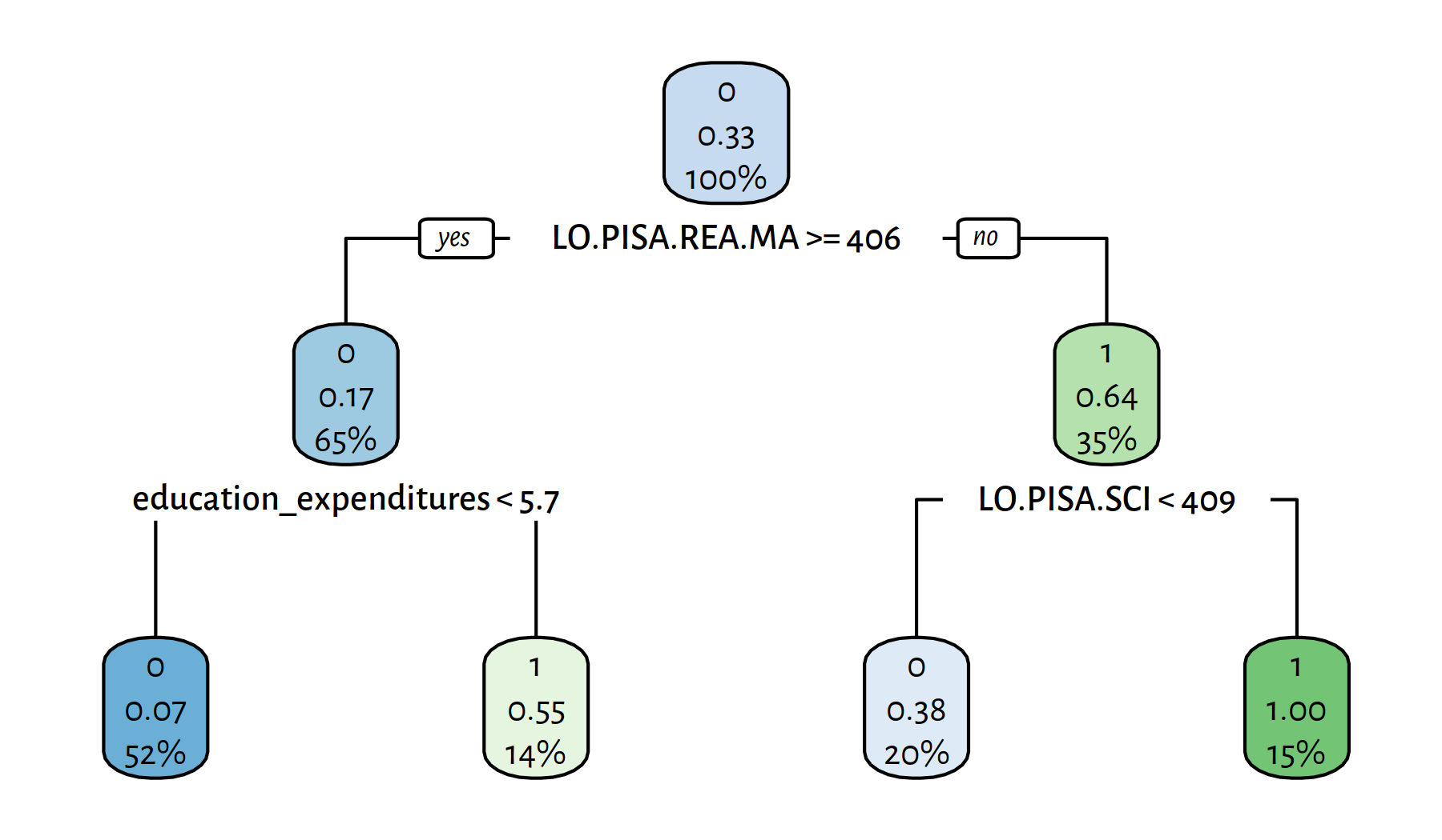
Figure 4.13: Yet another decision tree explaining the girls_rule_maths variable
Performance metrics:
Y_pred <- predict(tree, edbook_subset, type="class")
get_metrics(Y_pred, edbook_subset$girls_rule_maths)## Acc Prec Rec F TN FN FP TP
## 0.82716 0.78261 0.66667 0.72000 49.00000 9.00000 5.00000 18.00000The variables included in the model are:
This is… not at all enlightening. Rest assured that experts in education or econometrics for whom we work in this (imaginary) project would raise many questions at this very point. Merely applying some computational procedure on a dataset doesn’t cut it; it’s too early to ask for a paycheque. Classifiers are just blind tools in our gentle yet firm hands; new questions are risen, new answers must be sought. Further explorations are of course left as an exercise to the kind reader.
4.4.4 EdStats – Fitting of Binary Logistic Regression Models
In this task we’re going to consider the “wide” version of the EdStats dataset again:
edstats <- read.csv("datasets/edstats_2019_wide.csv",
comment.char="#")Let’s re-add the girls_rule_maths column
just as in the previous exercise.
Then, let’s create a subset of edstats that doesn’t include
the country names as well as the boys’ and girls’ math scores.
edstats$girls_rule_maths <-
factor(as.numeric(
edstats$LO.PISA.MAT.FE>edstats$LO.PISA.MAT.MA
))
edstats_subset <- edstats[!(names(edstats) %in%
c("CountryName", "LO.PISA.MAT.FE", "LO.PISA.MAT.MA"))]Fit and assess a logistic regression model for girls_rule_maths as a function
of LO.PISA.REA.MA+LO.PISA.SCI.
Click here for a solution.
Fitting of the model:
(f1 <- glm(girls_rule_maths~LO.PISA.REA.MA+LO.PISA.SCI,
data=edstats_subset, family=binomial("logit")))##
## Call: glm(formula = girls_rule_maths ~ LO.PISA.REA.MA + LO.PISA.SCI,
## family = binomial("logit"), data = edstats_subset)
##
## Coefficients:
## (Intercept) LO.PISA.REA.MA LO.PISA.SCI
## 3.0927 -0.0882 0.0755
##
## Degrees of Freedom: 80 Total (i.e. Null); 78 Residual
## (187 observations deleted due to missingness)
## Null Deviance: 103
## Residual Deviance: 77.9 AIC: 83.9Performance metrics:
Y_pred <- as.numeric(predict(f1, edstats_subset, type="response")>0.5)
get_metrics(Y_pred, edstats_subset$girls_rule_maths)## Acc Prec Rec F TN FN FP TP
## 0.79012 0.75000 0.55556 0.63830 49.00000 12.00000 5.00000 15.00000Relate the above numbers to those reported for the fitted decision trees.
Note that the fitted model is nicely interpretable:
the lower the boys’ average result on the Reading Scale
or the higher the country’s result on the Science Scale,
the higher the probability for girls_rule_maths:
example_X <- data.frame(
LO.PISA.REA.MA=c(475, 450, 475, 500),
LO.PISA.SCI= c(525, 525, 550, 500)
)
cbind(example_X,
`Pr(Y=1)`=predict(f1, example_X, type="response"))## LO.PISA.REA.MA LO.PISA.SCI Pr(Y=1)
## 1 475 525 0.703342
## 2 450 525 0.955526
## 3 475 550 0.939986
## 4 500 500 0.038094(*) Fit and assess a logistic regression model for girls_rule_maths
featuring all LO.PISA.REA* and LO.PISA.SCI* as independent variables.
Click here for a solution.
Model fitting:
(f2 <- glm(girls_rule_maths~LO.PISA.REA+LO.PISA.REA.FE+LO.PISA.REA.MA+
LO.PISA.SCI+LO.PISA.SCI.FE+LO.PISA.SCI.MA,
data=edstats_subset, family=binomial("logit")))## Warning: glm.fit: fitted probabilities numerically 0 or 1 occurred##
## Call: glm(formula = girls_rule_maths ~ LO.PISA.REA + LO.PISA.REA.FE +
## LO.PISA.REA.MA + LO.PISA.SCI + LO.PISA.SCI.FE + LO.PISA.SCI.MA,
## family = binomial("logit"), data = edstats_subset)
##
## Coefficients:
## (Intercept) LO.PISA.REA LO.PISA.REA.FE LO.PISA.REA.MA
## -2.265 1.268 -0.544 -0.734
## LO.PISA.SCI LO.PISA.SCI.FE LO.PISA.SCI.MA
## 1.269 -0.157 -1.112
##
## Degrees of Freedom: 80 Total (i.e. Null); 74 Residual
## (187 observations deleted due to missingness)
## Null Deviance: 103
## Residual Deviance: 33 AIC: 47The mysterious fitted probabilities numerically 0 or 1 occurred warning
denotes convergence problems of the underlying optimisation (fitting) procedure:
at least one of the model coefficients has had a fairly large order
of magnitude and hence the fitted probabilities has come very close to 0 or 1.
Recall that the probabilities are modelled by means of the logistic sigmoid
function applied on the output of a linear combination of the dependent variables.
Moreover, cross-entropy features a logarithm, and \(\log 0 = -\infty\).
This can be due to the fact that all the variables in the model are very correlated with each other (multicollinearity; an ill-conditioned problem). The obtained solution might be unstable – there might be many local optima and hence, different parameter vectors might be equally good. Moreover, it is likely that a small change in one of the inputs might lead to large change in the estimated model (* normally, we would attack this problem by employing some regularisation techniques).
Of course, the model’s performance metrics can still be computed, but then it’s better if we treat it as a black box. Or, even better, reduce the number of independent variables and come up with a simpler model that serves its purpose better than this one.
Y_pred <- as.numeric(predict(f2, edstats_subset, type="response")>0.5)
get_metrics(Y_pred, edstats_subset$girls_rule_maths)## Acc Prec Rec F TN FN FP TP
## 0.86420 0.83333 0.74074 0.78431 50.00000 7.00000 4.00000 20.000004.4.5 EdStats – Variable Selection in Binary Logistic Regression (*)
Back to our girls_rule_maths example, we still have so much to learn!
edstats <- read.csv("datasets/edstats_2019_wide.csv",
    comment.char="#")
edstats$girls_rule_maths <-
    factor(as.numeric(
        edstats$LO.PISA.MAT.FE>edstats$LO.PISA.MAT.MA
    ))
edstats_subset <- edstats[!(names(edstats) %in%
c("CountryName", "LO.PISA.MAT.FE", "LO.PISA.MAT.MA"))]Construct a binary logistic regression model via forward selection of variables.
Click here for a solution.
Just as in the linear regression case, we can rely on the step() function.
model_empty <- girls_rule_maths~1
(model_full <- formula(model.frame(girls_rule_maths~.,
    data=edstats_subset)))
## girls_rule_maths ~ HD.HCI.AMRT + HD.HCI.AMRT.FE + HD.HCI.AMRT.MA +
## HD.HCI.EYRS + HD.HCI.EYRS.FE + HD.HCI.EYRS.MA + HD.HCI.HLOS +
## HD.HCI.HLOS.FE + HD.HCI.HLOS.MA + HD.HCI.MORT + HD.HCI.MORT.FE +
## HD.HCI.MORT.MA + HD.HCI.OVRL + HD.HCI.OVRL.FE + HD.HCI.OVRL.MA +
## IT.CMP.PCMP.P2 + IT.NET.USER.P2 + LO.PISA.MAT + LO.PISA.REA +
## LO.PISA.REA.FE + LO.PISA.REA.MA + LO.PISA.SCI + LO.PISA.SCI.FE +
## LO.PISA.SCI.MA + NY.GDP.MKTP.CD + NY.GDP.PCAP.CD + NY.GDP.PCAP.PP.CD +
## NY.GNP.PCAP.CD + NY.GNP.PCAP.PP.CD + SE.COM.DURS + SE.PRM.CMPT.FE.ZS +
## SE.PRM.CMPT.MA.ZS + SE.PRM.CMPT.ZS + SE.PRM.ENRL.TC.ZS +
## SE.PRM.ENRR + SE.PRM.ENRR.FE + SE.PRM.ENRR.MA + SE.PRM.NENR +
## SE.PRM.NENR.FE + SE.PRM.NENR.MA + SE.PRM.PRIV.ZS + SE.SEC.ENRL.TC.ZS +
## SE.SEC.ENRR + SE.SEC.ENRR.FE + SE.SEC.ENRR.MA + SE.SEC.NENR +
## SE.SEC.NENR.MA + SE.SEC.PRIV.ZS + SE.TER.ENRR + SE.TER.ENRR.FE +
## SE.TER.ENRR.MA + SE.TER.PRIV.ZS + SE.XPD.TOTL.GD.ZS + SL.TLF.ADVN.FE.ZS +
## SL.TLF.ADVN.MA.ZS + SL.TLF.ADVN.ZS + SP.POP.TOTL + SP.POP.TOTL.FE.IN +
## SP.POP.TOTL.MA.IN + SP.PRM.TOTL.FE.IN + SP.PRM.TOTL.IN +
## SP.PRM.TOTL.MA.IN + SP.SEC.TOTL.FE.IN + SP.SEC.TOTL.IN +
## SP.SEC.TOTL.MA.IN + UIS.PTRHC.56 + UIS.SAP.CE + UIS.SAP.CE.F +
## UIS.SAP.CE.M + UIS.X.PPP.1.FSGOV + UIS.X.PPP.2T3.FSGOV +
## UIS.X.PPP.5T8.FSGOV + UIS.X.US.1.FSGOV + UIS.X.US.2T3.FSGOV +
## UIS.X.US.5T8.FSGOV + UIS.XGDP.1.FSGOV + UIS.XGDP.23.FSGOV +
## UIS.XGDP.56.FSGOV + UIS.XUNIT.GDPCAP.1.FSGOV + UIS.XUNIT.GDPCAP.23.FSGOV +
## UIS.XUNIT.GDPCAP.5T8.FSGOV + UIS.XUNIT.PPP.1.FSGOV.FFNTR +
## UIS.XUNIT.PPP.2T3.FSGOV.FFNTR + UIS.XUNIT.PPP.5T8.FSGOV.FFNTR +
## UIS.XUNIT.US.1.FSGOV.FFNTR + UIS.XUNIT.US.23.FSGOV.FFNTR +
## UIS.XUNIT.US.5T8.FSGOV.FFNTRf <- step(glm(model_empty, data=edstats_subset, family=binomial("logit")),
scope=model_full, direction="forward")## Start: AIC=105.12
## girls_rule_maths ~ 1## Error in model.matrix.default(Terms, m, contrasts.arg = object$contrasts): variable 1 has no levelsMelbourne, we have a problem!
Our dataset has too many missing values, and those cannot be present
in a logistic regression model (it’s based on a linear combination of variables,
and sums/products involving NAs yield NAs…).
Looking at the manual of ?step, we see that the default
NA handling is via na.omit(), and that, when applied on a data frame,
results in the removal of all the rows, where there is at least one NA.
Sadly, it’s too invasive.
We should get rid of the data blanks manually.
First, definitely, we should remove all the rows where
girls_rule_maths is unknown:
edstats_subset <-
    edstats_subset[!is.na(edstats_subset$girls_rule_maths),]
We are about to apply the forward selection process, whose purpose is to choose variables for a model. Therefore, instead of removing any more rows, we should remove the… columns with missing data:
edstats_subset <-
    edstats_subset[,colSums(sapply(edstats_subset, is.na))==0]
(*) Alternatively, we could apply some techniques of missing data imputation;
this is beyond the scope of this book. For instance, NAs could be
replaced by the averages of their respective columns.
We are ready now to make use of step().
model_empty <- girls_rule_maths~1
(model_full <- formula(model.frame(girls_rule_maths~.,
    data=edstats_subset)))
## girls_rule_maths ~ IT.NET.USER.P2 + LO.PISA.MAT + LO.PISA.REA +
## LO.PISA.REA.FE + LO.PISA.REA.MA + LO.PISA.SCI + LO.PISA.SCI.FE +
## LO.PISA.SCI.MA + NY.GDP.MKTP.CD + NY.GDP.PCAP.CD + SP.POP.TOTLf <- step(glm(model_empty, data=edstats_subset, family=binomial("logit")),
scope=model_full, direction="forward")## Start: AIC=105.12
## girls_rule_maths ~ 1
##
## Df Deviance AIC
## + LO.PISA.REA.MA 1 90.9 94.9
## + LO.PISA.SCI.MA 1 93.3 97.3
## + NY.GDP.MKTP.CD 1 94.2 98.2
## + LO.PISA.REA 1 95.0 99.0
## + LO.PISA.SCI 1 96.9 100.9
## + LO.PISA.MAT 1 97.2 101.2
## + LO.PISA.REA.FE 1 97.9 101.9
## + LO.PISA.SCI.FE 1 99.4 103.4
## <none> 103.1 105.1
## + SP.POP.TOTL 1 101.9 105.9
## + NY.GDP.PCAP.CD 1 102.3 106.3
## + IT.NET.USER.P2 1 103.1 107.1
##
## Step: AIC=94.93
## girls_rule_maths ~ LO.PISA.REA.MA
##
## Df Deviance AIC
## + LO.PISA.REA 1 42.8 48.8
## + LO.PISA.REA.FE 1 50.5 56.5
## + LO.PISA.SCI.FE 1 65.4 71.4
## + LO.PISA.SCI 1 77.9 83.9
## + LO.PISA.MAT 1 83.5 89.5
## + NY.GDP.MKTP.CD 1 87.4 93.4
## + IT.NET.USER.P2 1 87.5 93.5
## <none> 90.9 94.9
## + NY.GDP.PCAP.CD 1 89.2 95.2
## + LO.PISA.SCI.MA 1 89.2 95.2
## + SP.POP.TOTL 1 90.2 96.2
##
## Step: AIC=48.83
## girls_rule_maths ~ LO.PISA.REA.MA + LO.PISA.REA
##
## Df Deviance AIC
## <none> 42.8 48.8
## + LO.PISA.SCI.FE 1 40.9 48.9
## + SP.POP.TOTL 1 41.2 49.2
## + NY.GDP.PCAP.CD 1 41.3 49.3
## + LO.PISA.SCI 1 42.0 50.0
## + LO.PISA.MAT 1 42.4 50.4
## + IT.NET.USER.P2 1 42.7 50.7
## + LO.PISA.SCI.MA 1 42.7 50.7
## + NY.GDP.MKTP.CD 1 42.7 50.7
## + LO.PISA.REA.FE 1 42.8 50.8print(f)##
## Call: glm(formula = girls_rule_maths ~ LO.PISA.REA.MA + LO.PISA.REA,
## family = binomial("logit"), data = edstats_subset)
##
## Coefficients:
## (Intercept) LO.PISA.REA.MA LO.PISA.REA
## -0.176 -0.600 0.577
##
## Degrees of Freedom: 80 Total (i.e. Null); 78 Residual
## Null Deviance: 103
## Residual Deviance: 42.8 AIC: 48.8Y_pred <- as.numeric(predict(f, edstats_subset, type="response")>0.5)
get_metrics(Y_pred, edstats_subset$girls_rule_maths)## Acc Prec Rec F TN FN FP TP
## 0.88889 0.84615 0.81481 0.83019 50.00000 5.00000 4.00000 22.00000Choose a model via backward elimination.
Click here for a solution.
Having a dataset with missing values removed, this is easy now:
f <- suppressWarnings( # yeah, yeah, yeah...
# fitted probabilities numerically 0 or 1 occurred
step(glm(model_full, data=edstats_subset, family=binomial("logit")),
scope=model_empty, direction="backward")
)## Start: AIC=50.83
## girls_rule_maths ~ IT.NET.USER.P2 + LO.PISA.MAT + LO.PISA.REA +
##     LO.PISA.REA.FE + LO.PISA.REA.MA + LO.PISA.SCI + LO.PISA.SCI.FE +
##     LO.PISA.SCI.MA + NY.GDP.MKTP.CD + NY.GDP.PCAP.CD + SP.POP.TOTL
##
## Df Deviance AIC
## - LO.PISA.MAT 1 26.8 48.8
## - LO.PISA.SCI.MA 1 26.8 48.8
## - NY.GDP.PCAP.CD 1 26.9 48.9
## - LO.PISA.SCI 1 26.9 48.9
## - LO.PISA.SCI.FE 1 27.1 49.1
## - LO.PISA.REA.FE 1 27.4 49.4
## - LO.PISA.REA 1 27.5 49.5
## - LO.PISA.REA.MA 1 27.6 49.6
## <none> 26.8 50.8
## - IT.NET.USER.P2 1 29.3 51.3
## - NY.GDP.MKTP.CD 1 29.9 51.9
## - SP.POP.TOTL 1 31.7 53.7
##
## Step: AIC=48.84
## girls_rule_maths ~ IT.NET.USER.P2 + LO.PISA.REA + LO.PISA.REA.FE +
## LO.PISA.REA.MA + LO.PISA.SCI + LO.PISA.SCI.FE + LO.PISA.SCI.MA +
## NY.GDP.MKTP.CD + NY.GDP.PCAP.CD + SP.POP.TOTL
##
## Df Deviance AIC
## - LO.PISA.SCI.MA 1 26.8 46.8
## - NY.GDP.PCAP.CD 1 26.9 46.9
## - LO.PISA.SCI 1 27.0 47.0
## - LO.PISA.SCI.FE 1 27.1 47.1
## - LO.PISA.REA.FE 1 27.4 47.4
## - LO.PISA.REA 1 27.5 47.5
## - LO.PISA.REA.MA 1 27.6 47.6
## <none> 26.8 48.8
## - IT.NET.USER.P2 1 29.3 49.3
## - NY.GDP.MKTP.CD 1 29.9 49.9
## - SP.POP.TOTL 1 31.7 51.7
##
## Step: AIC=46.84
## girls_rule_maths ~ IT.NET.USER.P2 + LO.PISA.REA + LO.PISA.REA.FE +
## LO.PISA.REA.MA + LO.PISA.SCI + LO.PISA.SCI.FE + NY.GDP.MKTP.CD +
## NY.GDP.PCAP.CD + SP.POP.TOTL
##
## Df Deviance AIC
## - NY.GDP.PCAP.CD 1 26.9 44.9
## <none> 26.8 46.8
## - IT.NET.USER.P2 1 29.3 47.3
## - NY.GDP.MKTP.CD 1 29.9 47.9
## - LO.PISA.REA.FE 1 31.0 49.0
## - SP.POP.TOTL 1 31.8 49.8
## - LO.PISA.SCI 1 35.6 53.6
## - LO.PISA.SCI.FE 1 36.1 54.1
## - LO.PISA.REA 1 37.5 55.5
## - LO.PISA.REA.MA 1 50.9 68.9
##
## Step: AIC=44.87
## girls_rule_maths ~ IT.NET.USER.P2 + LO.PISA.REA + LO.PISA.REA.FE +
## LO.PISA.REA.MA + LO.PISA.SCI + LO.PISA.SCI.FE + NY.GDP.MKTP.CD +
## SP.POP.TOTL
##
## Df Deviance AIC
## <none> 26.9 44.9
## - NY.GDP.MKTP.CD 1 30.5 46.5
## - IT.NET.USER.P2 1 31.0 47.0
## - LO.PISA.REA.FE 1 31.1 47.1
## - SP.POP.TOTL 1 33.0 49.0
## - LO.PISA.SCI 1 35.9 51.9
## - LO.PISA.SCI.FE 1 36.4 52.4
## - LO.PISA.REA 1 37.5 53.5
## - LO.PISA.REA.MA 1 50.9 66.9The obtained model and its quality metrics:
print(f)##
## Call: glm(formula = girls_rule_maths ~ IT.NET.USER.P2 + LO.PISA.REA +
## LO.PISA.REA.FE + LO.PISA.REA.MA + LO.PISA.SCI + LO.PISA.SCI.FE +
## NY.GDP.MKTP.CD + SP.POP.TOTL, family = binomial("logit"),
## data = edstats_subset)
##
## Coefficients:
## (Intercept) IT.NET.USER.P2 LO.PISA.REA LO.PISA.REA.FE
## -1.66e+01 1.61e-01 1.85e+00 -8.00e-01
## LO.PISA.REA.MA LO.PISA.SCI LO.PISA.SCI.FE NY.GDP.MKTP.CD
## -1.03e+00 -1.35e+00 1.32e+00 -4.95e-12
## SP.POP.TOTL
## 6.20e-08
##
## Degrees of Freedom: 80 Total (i.e. Null); 72 Residual
## Null Deviance: 103
## Residual Deviance: 26.9 AIC: 44.9Y_pred <- as.numeric(predict(f, edstats_subset, type="response")>0.5)
get_metrics(Y_pred, edstats_subset$girls_rule_maths)## Acc Prec Rec F TN FN FP TP
## 0.91358 0.88462 0.85185 0.86792 51.00000 4.00000 3.00000 23.00000Note that we got a better (lower) AIC than in the forward selection
case, which means that backward elimination was better this time.
On the other hand, we needed to suppress the
fitted probabilities numerically 0 or 1 occurred warnings.
The returned model is perhaps unstable as well and consists of too
many variables.
4.5 Outro
4.5.1 Remarks
Other prominent classification algorithms:
- Naive Bayes and other probabilistic approaches,
- Support Vector Machines (SVMs) and other kernel methods,
- (Artificial) (Deep) Neural Networks.
Interestingly, in the next chapter we will note that the logistic regression model is a special case of a feed-forward single layer neural network.
We will also generalise the binary logistic regression to the case of a multiclass classification.
The state-of-the art classifiers called Random Forests and XGBoost (see also: AdaBoost) are based on decision trees. They tend to be more accurate but – at the same time – they fail to exhibit the decision trees’ important feature: interpretability.
Trees can also be used for regression tasks, see R package rpart.
4.5.2 Further Reading
Recommended further reading: (James et al. 2017: Chapters 4 and 8)
Other: (Hastie et al. 2017: Chapters 4 and 7 as well as (*) Chapters 9, 10, 13, 15)