3 Classification with K-Nearest Neighbours

These lecture notes are distributed in the hope that they will be useful. Any bug reports are appreciated.

3.1 Introduction

3.1.1 Classification Task

Let \(\mathbf{X}\in\mathbb{R}^{n\times p}\) be an input matrix that consists of \(n\) points in a \(p\)-dimensional space (each of the \(n\) objects is described by means of \(p\) numerical features).

Recall that in supervised learning, with each \(\mathbf{x}_{i,\cdot}\) we associate the desired output \(y_i\).

\[ \mathbf{X}= \left[ \begin{array}{cccc} x_{1,1} & x_{1,2} & \cdots & x_{1,p} \\ x_{2,1} & x_{2,2} & \cdots & x_{2,p} \\ \vdots & \vdots & \ddots & \vdots \\ x_{n,1} & x_{n,2} & \cdots & x_{n,p} \\ \end{array} \right] \qquad \mathbf{y} = \left[ \begin{array}{c} {y}_{1} \\ {y}_{2} \\ \vdots\\ {y}_{n} \\ \end{array} \right]. \]

In this chapter we are interested in classification tasks; we assume that each \(y_i\) is a label (e.g., a character string) – it is of quantitative/categorical type.

Most commonly, we are faced with binary classification tasks where there are only two possible distinct labels.

We traditionally denote them with \(0\)s and \(1\)s.

For example:

0	1
no	yes
false	true
failure	success
healthy	ill

On the other hand, in multiclass classification, we assume that each \(y_i\) takes more than two possible values.

Example plot of a synthetic dataset with the reference binary \(y\)s is given in Figure 3.1. The “true” decision boundary is at \(X_1=0\) but the classes slightly overlap (the dataset is a bit noisy).

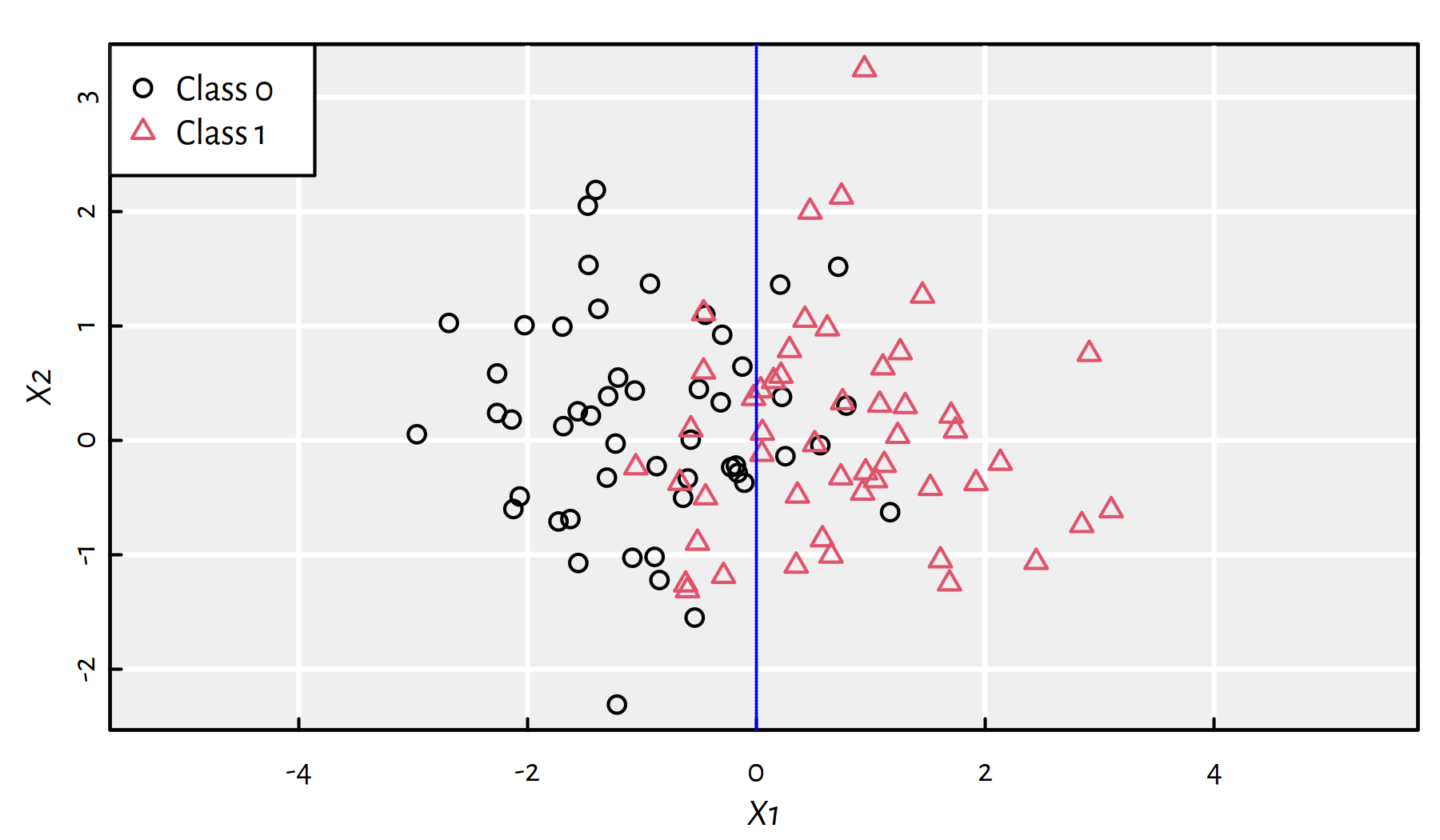
Figure 3.1: A synthetic 2D dataset with the true decision boundary at \(X_1=0\)

3.1.2 Data

For illustration, let’s consider the Wine Quality dataset (Cortez et al. 2009) that can be downloaded from the UCI Machine Learning Repository (https://archive.ics.uci.edu/ml/datasets/Wine+Quality) – white wines only.

wines <- read.csv("datasets/winequality-all.csv",
    comment.char="#")
wines <- wines[wines$color == "white",]
(n <- nrow(wines)) # number of samples

## [1] 4898

These are Vinho Verde wine samples from the north of Portugal, see https://www.vinhoverde.pt/en/homepage.

There are 11 physicochemical features reported. Moreover, there is a wine rating (which we won’t consider here) on the scale 0 (bad) to 10 (excellent) given by wine experts.

The input matrix \(\mathbf{X}\in\mathbb{R}^{n\times p}\) consists of the first 10 numeric variables:

X <- as.matrix(wines[,1:10])
dim(X)

## [1] 4898   10

head(X, 2) # first two rows

##      fixed.acidity volatile.acidity citric.acid residual.sugar
## 1600           7.0             0.27        0.36           20.7
## 1601           6.3             0.30        0.34            1.6
##      chlorides free.sulfur.dioxide total.sulfur.dioxide density  pH
## 1600     0.045                  45                  170   1.001 3.0
## 1601     0.049                  14                  132   0.994 3.3
##      sulphates
## 1600      0.45
## 1601      0.49

The 11th variable measures the amount of alcohol (in %).

We will convert this dependent variable to a binary one:

0 == (alcohol < 12) == lower-alcohol wines1
1 == (alcohol >= 12) == higher-alcohol wines

# recall that TRUE == 1
Y <- factor(as.character(as.numeric(wines$alcohol >= 12)))
table(Y)

## Y
##    0    1 
## 4085  813

Now \((\mathbf{X},\mathbf{y})\) is a basis for an interesting (yet challenging) binary classification task.

3.1.3 Training and Test Sets

Recall that we are genuinely interested in the construction of supervised learning models for the two following purposes:

description – to explain a given dataset in simpler terms,
prediction – to forecast the values of the dependent variable for inputs that are yet to be observed.

In the latter case:

we don’t want our models to overfit to current data,
we want our models to generalise well to new data.

One way to assess if a model has sufficient predictive power is based on a random train-test split of the original dataset:

training sample (usually 60-80% of the observations) – used to construct a model,
test sample (remaining 40-20%) – used to assess the goodness of fit.

Remark.: Test sample must not be used in the training phase! (No cheating!)

60/40% train-test split in R:

set.seed(123) # reproducibility matters
random_indices <- sample(n)
head(random_indices) # preview

## [1] 2463 2511 2227  526 4291 2986

# first 60% of the indices (they are arranged randomly)
# will constitute the train sample:
train_indices <- random_indices[1:floor(n*0.6)]
X_train <- X[train_indices,]
Y_train <- Y[train_indices]
# the remaining indices (40%) go to the test sample:
X_test  <- X[-train_indices,]
Y_test  <- Y[-train_indices]

3.1.4 Discussed Methods

Our aim is to build a classifier that takes 10 wine physicochemical features and determines whether it’s a “strong” wine.

We will discuss 3 simple and educational (yet practically useful) classification algorithms:

K-nearest neighbour scheme – this chapter,
Decision trees – the next chapter,
Logistic regression – the next chapter.

3.2 K-nearest Neighbour Classifier

3.2.1 Introduction

Rule.: “If you don’t know what to do in a situation, just act like the people around you”

For some integer \(K\ge 1\), the K-Nearest Neighbour (K-NN) Classifier proceeds as follows.

To classify a new point \(\mathbf{x}'\):

find the \(K\) nearest neighbours of a given point \(\mathbf{x}'\) amongst the points in the train set, denoted \(\mathbf{x}_{i_1,\cdot}, \dots, \mathbf{x}_{i_K,\cdot}\):
1. compute the Euclidean distances between \(\mathbf{x}'\) and each \(\mathbf{x}_{i,\cdot}\) from the train set, \[d_i = \|\mathbf{x}'-\mathbf{x}_{i,\cdot}\|\]
2. order \(d_i\)s in increasing order, \(d_{i_1} \le d_{i_2} \le \dots \le d_{i_K}\)
3. pick first \(K\) indices (these are the nearest neighbours)
fetch the corresponding reference labels \(y_{i_1}, \dots, y_{i_K}\)
return their mode as a result, i.e., the most frequently occurring label (a.k.a. majority vote)

Here is how \(K\)-NN classifier works on a synthetic 2D dataset. Firstly let’s consider \(K=1\), see Figure 3.2. Gray and pink regions depict how new points would be classified. In particular 1-NN is “greedy” in the sense that we just locate the nearest point.

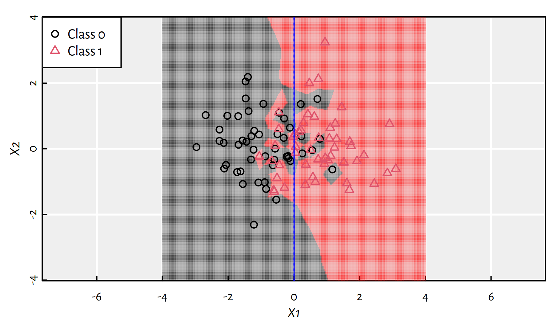
Figure 3.2: 1-NN class bounds for our 2D synthetic dataset

Remark.: (*) 1-NN classification is essentially based on a dataset’s so-called Voronoi diagram.

Increasing \(K\) somehow smoothens the decision boundary (this makes it less “local” and more “global”). Figure 3.3 depicts the \(K=3\) case.

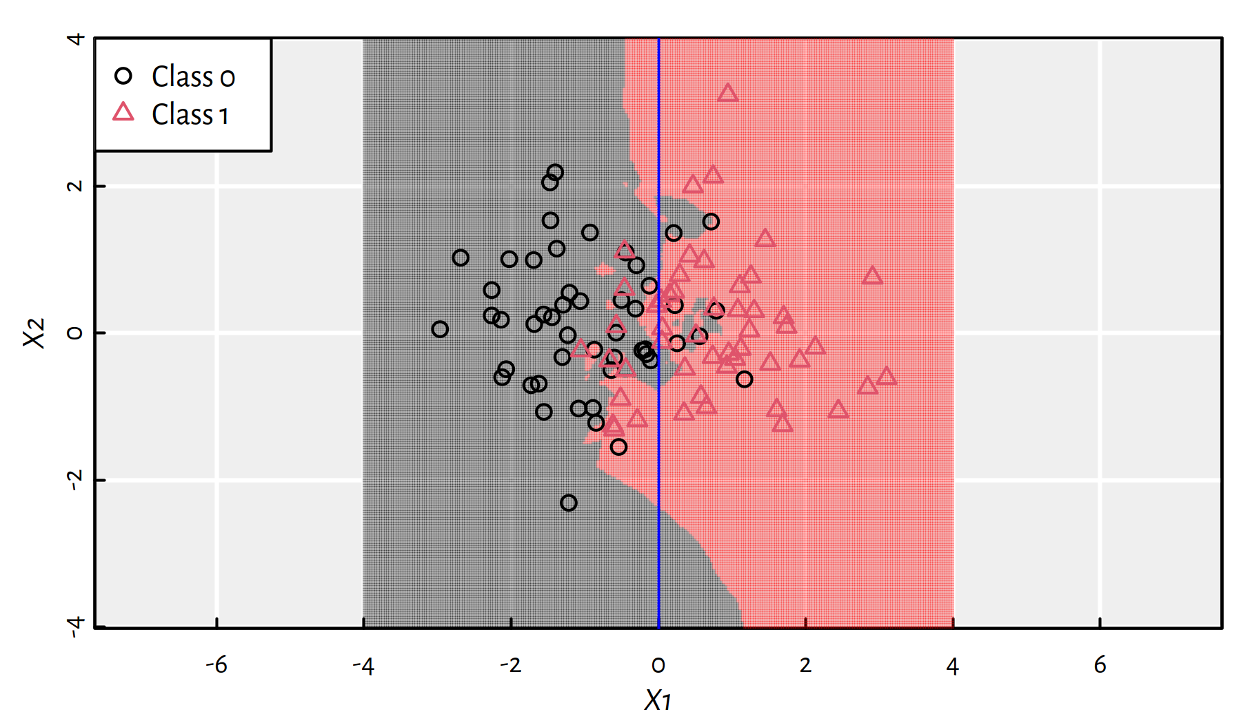
Figure 3.3: 3-NN class bounds for our 2D synthetic dataset

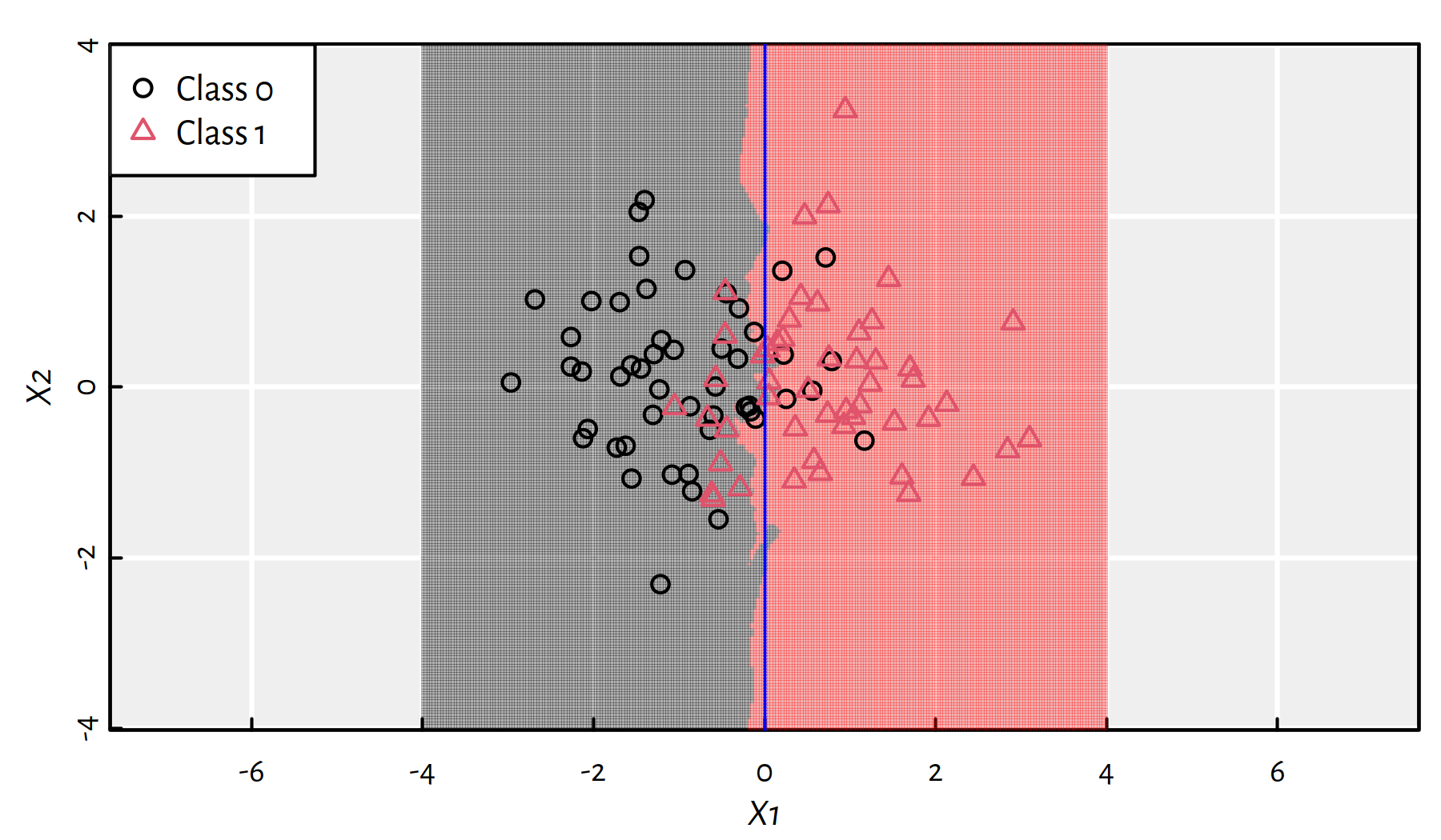
Figure 3.4: 25-NN class bounds for our 2D synthetic dataset

Recall that the “true” decision boundary for this synthetic dataset is at \(X_1=0\). The 25-NN classifier did quite a good job, see Figure 3.4.

3.2.2 Example in R

We shall be calling the knn() function from package FNN to classify the points from the test sample extracted from the wines dataset:

library("FNN")

Let’s make prediction using the 5-nn classifier:

Y_knn5 <- knn(X_train, X_test, Y_train, k=5)
head(Y_test, 28) # True Ys

##  [1] 0 0 0 0 0 1 0 0 0 0 0 0 0 0 0 0 0 0 0 0 0 0 0 0 0 0 0 0
## Levels: 0 1

head(Y_knn5, 28) # Predicted Ys

##  [1] 1 1 0 0 0 0 0 0 0 0 0 0 0 0 0 0 0 0 0 0 0 0 0 0 0 0 0 0
## Levels: 0 1

mean(Y_test == Y_knn5) # accuracy

## [1] 0.81735

9-nn classifier:

Y_knn9 <- knn(X_train, X_test, Y_train, k=9)
head(Y_test, 28) # True Ys

##  [1] 0 0 0 0 0 1 0 0 0 0 0 0 0 0 0 0 0 0 0 0 0 0 0 0 0 0 0 0
## Levels: 0 1

head(Y_knn9, 28) # Predicted Ys

##  [1] 0 0 0 0 0 0 0 0 0 0 0 0 0 1 0 0 0 0 0 0 0 0 0 0 0 0 0 0
## Levels: 0 1

mean(Y_test == Y_knn9) # accuracy

## [1] 0.81939

3.2.3 Feature Engineering

Note that the Euclidean distance that we used above implicitly assumes that every feature (independent variable) is on the same scale.

However, when dealing with, e.g., physical quantities, we often perform conversions of units of measurement (kg → g, feet → m etc.).

Transforming a single feature may drastically change the metric structure of the dataset and therefore highly affect the obtained predictions.

To “bring data to the same scale”, we often apply a trick called standardisation.

Computing the so-called Z-scores of the \(j\)-th feature, \(\mathbf{x}_{\cdot,j}\), is done by subtracting from each observation the sample mean and dividing the result by the sample standard deviation:

\[z_{i,j} = \frac{x_{i,j}-\bar{x}_{\cdot,j}}{s_{x_{\cdot,j}}}\]

This a new feature \(\mathbf{z}_{\cdot,j}\) that always has mean 0 and standard deviation of 1.

Moreover, it is unit-less (e.g., we divide a value in kgs by a value in kgs, the units are cancelled out). This, amongst others, prevents one of the features from dominating the other ones.

Z-scores are easy to interpret, e.g., 0.5 denotes an observation that is 0.5 standard deviations above the mean and -3 informs us that a value is 3 standard deviations below the mean.

Remark.: (*) If data are normally distributed (bell-shaped histogram), with very high probability, most (expected value is 99.74%) observations should have Z-scores between -3 and 3. Those that don’t, are “suspicious”, maybe they are outliers? We should inspect them manually.

Let’s compute Z_train and Z_test, being the standardised versions of X_train and X_test, respectively.

means <- apply(X_train, 2, mean) # column means
sds   <- apply(X_train, 2, sd)   # column standard deviations
Z_train <- X_train # copy
Z_test  <- X_test  # copy
for (j in 1:ncol(X)) {
    Z_train[,j] <- (Z_train[,j]-means[j])/sds[j]
    Z_test[,j]  <- (Z_test[,j] -means[j])/sds[j]
}

Note that we have transformed the training and test sample in the very same way. Computing means and standard deviations separately for these two datasets is a common error – it is the training set that we use in the course of the learning process. The above can be re-written as:

Z_train <- t(apply(X_train, 1, function(r) (r-means)/sds))
Z_test  <- t(apply(X_test,  1, function(r) (r-means)/sds))

See Figure 3.5 for an illustration. Note that the righthand figures (histograms of standardised variables) are on the same scale now.

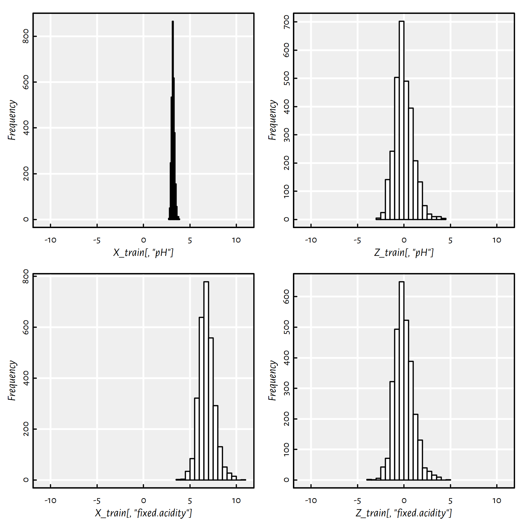
Figure 3.5: Empirical distribution of two variables (pH on the top, fixed.acidity on the bottom) before (left) and after (right) standardising

Remark.: Of course, standardisation is only about shifting and scaling, it preserves the shape of the distribution. If the original variable is right skewed or bimodal, its standardised version will remain as such.

Let’s compute the accuracy of K-NN classifiers acting on standardised data.

Y_knn5s <- knn(Z_train, Z_test, Y_train, k=5)
mean(Y_test == Y_knn5s) # accuracy

## [1] 0.91429

Y_knn9s <- knn(Z_train, Z_test, Y_train, k=9)
mean(Y_test == Y_knn9s) # accuracy

## [1] 0.91378

The accuracy is much better.

Standardisation is an example of feature engineering.

Good models rarely work well “straight out of the box” – if that was the case, we wouldn’t need data scientists and machine learning engineers!

To increase models’ accuracy, we often spend a lot of time:

cleansing data (e.g., removing outliers)
extracting new features
transforming existing features
trying to find a set of features that are relevant

This is the “more art than science” part of data science (sic!), and hence most textbooks are not really eager for discussing such topics (including this one).

Sorry, this is sad but true. The solutions that work well in the case of dataset A may fail in the B case and vice versa. However, the more exercises you solve, the greater the arsenal of ideas/possible approaches you will have at hand when dealing with real-world problems.

Feature selection – example (manually selected columns):

features <- c("density", "residual.sugar")
Y_knn5s <- knn(Z_train[,features], Z_test[,features],
    Y_train, k=5)
mean(Y_test == Y_knn5s) # accuracy

## [1] 0.91633

Y_knn9s <- knn(Z_train[,features], Z_test[,features],
    Y_train, k=9)
mean(Y_test == Y_knn9s) # accuracy

## [1] 0.925

Exercise.

Try to find a combination of 2-4 features (by guessing or applying magic tricks) that increases the accuracy of a \(K\)-NN classifier on this dataset.

3.3 Model Assessment and Selection

3.3.1 Performance Metrics

Recall that \(y_i\) denotes the true label associated with the \(i\)-th observation.

Let \(\hat{y}_i\) denote the classifier’s output for a given \(\mathbf{x}_{i,\cdot}\).

Ideally, we’d wish that \(\hat{y}_i=y_i\).

Sadly, in practice we will make errors.

Here are the 4 possible situations (true vs. predicted label):

.	\(y_i=0\)	\(y_i=1\)
\(\hat{y}_i=0\)	True Negative	False Negative (Type II error)
\(\hat{y}_i=1\)	False Positive (Type I error)	True Positive

Note that the terms positive and negative refer to the classifier’s output, i.e., occur when \(\hat{y}_i\) is equal to \(1\) and \(0\), respectively.

A confusion matrix is used to summarise the correctness of predictions for the whole sample:

Y_pred <- knn(Z_train, Z_test, Y_train, k=9)
(C <- table(Y_pred, Y_test))

##       Y_test
## Y_pred    0    1
##      0 1607  133
##      1   36  184

For example,

C[1,1] # number of TNs

## [1] 1607

C[2,1] # number of FPs

## [1] 36

Accuracy is the ratio of the correctly classified instances to all the instances.

In other words, it is the probability of making a correct prediction.

\[ \text{Accuracy} = \frac{\text{TP}+\text{TN}}{\text{TP}+\text{TN}+\text{FP}+\text{FN}} = \frac{1}{n} \sum_{i=1}^n \mathbb{I}\left( y_i = \hat{y}_i \right) \] where \(\mathbb{I}\) is the indicator function, \(\mathbb{I}(l)=1\) if logical condition \(l\) is true and \(0\) otherwise.

mean(Y_test == Y_pred) # accuracy

## [1] 0.91378

(C[1,1]+C[2,2])/sum(C) # equivalently

## [1] 0.91378

In many applications we are dealing with unbalanced problems, where the case \(y_i=1\) is relatively rare, yet predicting it correctly is much more important than being accurate with respect to class \(0\).

Remark.: Think of medical applications, e.g., HIV testing or tumour diagnosis.

In such a case, accuracy as a metric fails to quantify what we are aiming for.

Remark.: If only 1% of the cases have true \(y_i=1\), then a dummy classifier that always outputs \(\hat{y}_i=0\) has 99% accuracy.

Metrics such as precision and recall (and their aggregated version, F-measure) aim to address this problem.

Precision

\[ \text{Precision} = \frac{\text{TP}}{\text{TP}+\text{FP}} \]

If the classifier outputs \(1\), what is the probability that this is indeed true?

C[2,2]/(C[2,2]+C[2,1]) # Precision

## [1] 0.83636

Recall (a.k.a. sensitivity, hit rate or true positive rate)

\[ \text{Recall} = \frac{\text{TP}}{\text{TP}+\text{FN}} \]

If the true class is \(1\), what is the probability that the classifier will detect it?

C[2,2]/(C[2,2]+C[1,2]) # Recall

## [1] 0.58044

Remark.: Precision or recall? It depends on an application. Think of medical diagnosis, medical screening, plagiarism detection, etc. — which measure is more important in each of the settings listed?

As a compromise, we can use the F-measure (a.k.a. \(F_1\)-measure), which is the harmonic mean of precision and recall:

\[ \text{F} = \frac{1}{ \frac{ \frac{1}{\text{Precision}}+\frac{1}{\text{Recall}} }{2} } = \left( \frac{1}{2} \left( \text{Precision}^{-1}+\text{Recall}^{-1} \right) \right)^{-1} = \frac{\text{TP}}{\text{TP} + \frac{\text{FP} + \text{FN}}{2}} \]

Exercise.

Show that the above equality holds.

C[2,2]/(C[2,2]+0.5*C[1,2]+0.5*C[2,1]) # F

## [1] 0.68529

The following function can come in handy in the future:

get_metrics <- function(Y_pred, Y_test)
{
    C <- table(Y_pred, Y_test) # confusion matrix
    stopifnot(dim(C) == c(2, 2))
    c(Acc=(C[1,1]+C[2,2])/sum(C), # accuracy
      Prec=C[2,2]/(C[2,2]+C[2,1]), # precision
      Rec=C[2,2]/(C[2,2]+C[1,2]), # recall
      F=C[2,2]/(C[2,2]+0.5*C[1,2]+0.5*C[2,1]), # F-measure
      # Confusion matrix items:
      TN=C[1,1], FN=C[1,2],
      FP=C[2,1], TP=C[2,2]
    ) # return a named vector
}

get_metrics(Y_pred, Y_test)

##        Acc       Prec        Rec          F         TN         FN 
##    0.91378    0.83636    0.58044    0.68529 1607.00000  133.00000 
##         FP         TP 
##   36.00000  184.00000

3.3.2 How to Choose K for K-NN Classification?

We haven’t yet considered the question which \(K\) yields the best classifier.

Best == one that has the highest predictive power.

Best == with respect to some chosen metric (accuracy, recall, precision, F-measure, …)

Let’s study how the metrics on the test set change as functions of the number of nearest neighbours considered, \(K\).

Auxiliary function:

knn_metrics <- function(k, X_train, X_test, Y_train, Y_test)
{
    Y_pred <- knn(X_train, X_test, Y_train, k=k) # classify
    get_metrics(Y_pred, Y_test)
}

For example:

knn_metrics(5, Z_train, Z_test, Y_train, Y_test)

##        Acc       Prec        Rec          F         TN         FN 
##    0.91429    0.82251    0.59937    0.69343 1602.00000  127.00000 
##         FP         TP 
##   41.00000  190.00000

Example call to evaluate metrics as a function of different \(K\)s:

Ks <- seq(1, 19, by=2)
Ps <- as.data.frame(t(
    sapply(Ks, # on each element in this vector
        knn_metrics,     # apply this function
        Z_train, Z_test, Y_train, Y_test # aux args
    )))

Remark.: Note that sapply(X, f, arg1, arg2, ...) outputs a list Y such that Y[[i]] = f(X[i], arg1, arg2, ...) which is then simplified to a matrix.
Remark.: We transpose this result, t(), in order to get each metric corresponding to different columns in the result. As usual, if you keep wondering, e.g., why t(), play with the code yourself – it’s fun fun fun.

Example results:

round(cbind(K=Ks, Ps), 2)

##     K  Acc Prec  Rec    F   TN  FN FP  TP
## 1   1 0.92 0.77 0.72 0.74 1574  90 69 227
## 2   3 0.92 0.79 0.66 0.72 1587 108 56 209
## 3   5 0.91 0.82 0.60 0.69 1602 127 41 190
## 4   7 0.91 0.82 0.56 0.67 1604 138 39 179
## 5   9 0.91 0.84 0.58 0.69 1607 133 36 184
## 6  11 0.91 0.85 0.56 0.68 1611 138 32 179
## 7  13 0.91 0.83 0.57 0.68 1606 136 37 181
## 8  15 0.91 0.83 0.55 0.66 1607 144 36 173
## 9  17 0.91 0.82 0.53 0.64 1607 149 36 168
## 10 19 0.90 0.81 0.52 0.63 1603 151 40 166

Figure 3.6 is worth a thousand tables though (see ?matplot in R). The reader is kindly asked to draw conclusions themself.

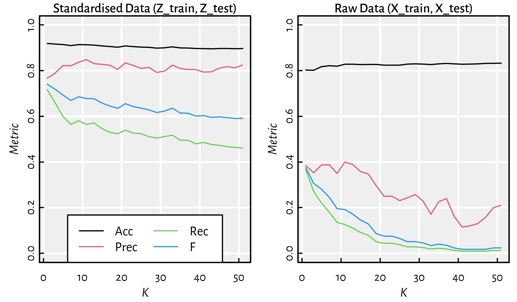
Figure 3.6: Performance of \(K\)-nn classifiers as a function of \(K\) for standardised and raw data

3.3.3 Training, Validation and Test sets

In the \(K\)-NN classification task, there are many hyperparameters to tune up:

Which \(K\) should we choose?
Should we standardise the dataset?
Which variables should be taken into account when computing the Euclidean distance?

Remark.: If we select the best hyperparameter set based on test sample error, we will run into the trap of overfitting again. This time we’ll be overfitting to the test set — the model that is optimal for a given test sample doesn’t have to generalise well to other test samples (!).

In order to overcome this problem, we can perform a random train-validation-test split of the original dataset:

training sample (e.g., 60%) – used to construct the models
validation sample (e.g., 20%) – used to tune the hyperparameters of the classifier
test sample (e.g., 20%) – used to assess the goodness of fit

An example way to perform a 60/20/20% train-validation-test split:

set.seed(123) # reproducibility matters
random_indices <- sample(n)
n1 <- floor(n*0.6)
n2 <- floor(n*0.8)
X2_train <- X[random_indices[1     :n1], ]
Y2_train <- Y[random_indices[1     :n1]  ]
X2_valid <- X[random_indices[(n1+1):n2], ]
Y2_valid <- Y[random_indices[(n1+1):n2]  ]
X2_test  <- X[random_indices[(n2+1):n ], ]
Y2_test  <- Y[random_indices[(n2+1):n ]  ]
stopifnot(nrow(X2_train)+nrow(X2_valid)+nrow(X2_test)
    == nrow(X))

Exercise.

Find the best \(K\) on the validation set and compute the error metrics on the test set.

Remark.: (*) If our dataset is too small, we can use various cross-validation techniques instead of a train-validate-test split.

3.4 Implementing a K-NN Classifier (*)

3.4.1 Factor Data Type

Recall that (see Appendix B for more details) factor type in R is a very convenient means to encode categorical data (such as \(\mathbf{y}\)):

x <- c("yes", "no", "no", "yes", "no")
f <- factor(x, levels=c("no", "yes"))
f

## [1] yes no  no  yes no 
## Levels: no yes

table(f) # counts

## f
##  no yes 
##   3   2

Internally, objects of type factor are represented as integer vectors with elements in \(\{1,\dots,M\}\), where \(M\) is the number of possible levels.

Labels, used to “decipher” the numeric codes, are stored separately.

as.numeric(f) # 2nd label, 1st label, 1st label etc.

## [1] 2 1 1 2 1

levels(f)

## [1] "no"  "yes"

levels(f) <- c("failure", "success") # re-encode
f

## [1] success failure failure success failure
## Levels: failure success

3.4.2 Main Routine (*)

Let’s implement a K-NN classifier ourselves by using a top-bottom approach.

We will start with a general description of the admissible inputs and the expected output.

Then we will arrange the processing of data into conveniently manageable chunks.

The function’s declaration will look like:

our_knn <- function(X_train, X_test, Y_train, k=1) {
    # k=1 denotes a parameter with a default value
    # ...
}

Load an example dataset on which we will test our algorithm:

wines <- read.csv("datasets/winequality-all.csv",
    comment.char="#")
wines <- wines[wines$color == "white",]
X <- as.matrix(wines[,1:10])
Y <- factor(as.character(as.numeric(wines$alcohol >= 12)))

Note that Y is now a factor object.

Train-test split:

set.seed(123)
random_indices <- sample(n)
train_indices <- random_indices[1:floor(n*0.6)]
X_train <- X[train_indices,]
Y_train <- Y[train_indices]
X_test  <- X[-train_indices,]
Y_test  <- Y[-train_indices]

First, we should specify the type and form of the arguments we’re expecting:

# this is the body of our_knn() - part 1
stopifnot(is.numeric(X_train), is.matrix(X_train))
stopifnot(is.numeric(X_test), is.matrix(X_test))
stopifnot(is.factor(Y_train))
stopifnot(ncol(X_train) == ncol(X_test))
stopifnot(nrow(X_train) == length(Y_train))
stopifnot(k >= 1)
n_train <- nrow(X_train)
n_test  <- nrow(X_test)
p <- ncol(X_train)
M <- length(levels(Y_train))

Therefore,

\(\mathtt{X\_train}\in\mathbb{R}^{\mathtt{n\_train}\times \mathtt{p}}\), \(\mathtt{X\_test}\in\mathbb{R}^{\mathtt{n\_test}\times \mathtt{p}}\) and \(\mathtt{Y\_train}\in\{1,\dots,M\}^{\mathtt{n\_train}}\)

Remark.: Recall that R factor objects are internally encoded as integer vectors.

Next, we will call the (to-be-done) function our_get_knnx(), which seeks nearest neighbours of all the points:

# our_get_knnx returns a matrix nn_indices of size n_test*k,
# where nn_indices[i,j] denotes the index of
# X_test[i,]'s j-th nearest neighbour in X_train.
# (It is the point X_train[nn_indices[i,j],]).
nn_indices <- our_get_knnx(X_train, X_test, k)

Then, for each point in X_test, we fetch the labels corresponding to its nearest neighbours and compute their mode:

Y_pred <- numeric(n_test) # vector of length n_test
# For now we will operate on the integer labels in {1,...,M}
Y_train_int <- as.numeric(Y_train)
for (i in 1:n_test) {
    # Get the labels of the NNs of the i-th point:
    nn_labels_i <- Y_train_int[nn_indices[i,]]
    # Compute the mode (majority vote):
    Y_pred[i] <- our_mode(nn_labels_i) # in {1,...,M}
}

Finally, we should convert the resulting integer vector to an object of type factor:

# Convert Y_pred to factor:
return(factor(Y_pred, labels=levels(Y_train)))

3.4.3 Mode

To implement the mode, we can use the tabulate() function.

Exercise.

Read the function’s man page, see ?tabulate.

For example:

tabulate(c(1, 2, 1, 1, 1, 5, 2))

## [1] 4 2 0 0 1

There might be multiple modes – in such a case, we should pick one at random.

For that, we can use the sample() function.

Exercise.

Read the function’s man page, see ?sample. Note that its behaviour is different when it’s first argument is a vector of length 1.

An example implementation:

our_mode <- function(Y) {
    # tabulate() will take care of
    # checking the correctness of Y
    t <- tabulate(Y)
    mode_candidates <- which(t == max(t))
    if (length(mode_candidates) == 1) return(mode_candidates)
    else return(sample(mode_candidates, 1))
}

our_mode(c(1, 1, 1, 1))

## [1] 1

our_mode(c(2, 2, 2, 2))

## [1] 2

our_mode(c(3, 1, 3, 3))

## [1] 3

our_mode(c(1, 1, 3, 3, 2))

## [1] 3

our_mode(c(1, 1, 3, 3, 2))

## [1] 1

3.4.4 NN Search Routines (*)

Last but not least, we should implement the our_get_knnx() function.

It is the function responsible for seeking the indices of nearest neighbours.

It turns out this function will actually constitute the K-NN classifier’s performance bottleneck in case of big data samples.

# our_get_knnx returns a matrix nn_indices of size n_test*k,
# where nn_indices[i,j] denotes the index of
# X_test[i,]'s j-th nearest neighbour in X_train.
# (It is the point X_train[nn_indices[i,j],]).
our_get_knnx <- function(X_train, X_test, k) {
    # ...
}

A naive approach to our_get_knnx() relies on computing all pairwise distances, and sorting them.

our_get_knnx <- function(X_train, X_test, k) {
    n_test <- nrow(X_test)
    nn_indices <- matrix(NA_real_, nrow=n_test, ncol=k)
    for (i in 1:n_test) {
        d <- apply(X_train, 1, function(x)
            sqrt(sum((x-X_test[i,])^2)))
        # now d[j] is the distance
        # between X_train[j,] and X_test[i,]
        nn_indices[i,] <- order(d)[1:k]
    }
    nn_indices
}

A comparison with FNN:knn():

system.time(Ya <- knn(X_train, X_test, Y_train, k=5))

##    user  system elapsed 
##   0.128   0.000   0.128

system.time(Yb <- our_knn(X_train, X_test, Y_train, k=5))

##    user  system elapsed 
##  15.683   0.000  15.683

mean(Ya == Yb) # 1.0 on perfect match

## [1] 1

Both functions return identical results but our implementation is “slightly” slower.

FNN:knn() is efficiently written in C++, which is a compiled programming language.

R, on the other hand (just like Python and Matlab) is interpreted, therefore as a rule of thumb we should consider it an order of magnitude slower (see, however, the Julia language).

Let’s substitute our naive implementation with the equivalent one, but written in C++ (available in the FNN package).

Remark.: (*) Note that we can write a C++ implementation ourselves, see the Rcpp package for seamless R and C++ integration.

our_get_knnx <- function(X_train, X_test, k) {
    # this is used by our_knn()
    FNN::get.knnx(X_train, X_test, k, algorithm="brute")$nn.index
}
system.time(Ya <- knn(X_train, X_test, Y_train, k=5))

##    user  system elapsed 
##   0.124   0.000   0.124

system.time(Yb <- our_knn(X_train, X_test, Y_train, k=5))

##    user  system elapsed 
##   0.044   0.000   0.045

mean(Ya == Yb) # 1.0 on perfect match

## [1] 1

Note that our solution requires \(c\cdot n_\text{test}\cdot n_\text{train}\cdot p\) arithmetic operations for some \(c>1\). The overall cost of sorting is at least \(d\cdot n_\text{test}\cdot n_\text{train}\cdot\log n_\text{train}\) for some \(d>1\).

This does not scale well with both \(n_\text{test}\) and \(n_\text{train}\) (think – big data).

It turns out that there are special spatial data structures – such as metric trees – that aim to speed up searching for nearest neighbours in low-dimensional spaces (for small \(p\)).

Remark.: (*) Searching in high-dimensional spaces is hard due to the so-called curse of dimensionality.

For example, FNN::get.knnx() also implements the so-called kd-trees.

library("microbenchmark")
test_speed <- function(n, p, k) {
    A <- matrix(runif(n*p), nrow=n, ncol=p)
    s <- summary(microbenchmark::microbenchmark(
        brute=FNN::get.knnx(A, A, k, algorithm="brute"),
        kd_tree=FNN::get.knnx(A, A, k, algorithm="kd_tree"),
        times=3
    ), unit="s")
    # minima of 3 time measurements:
    structure(s$min, names=as.character(s$expr))
}

test_speed(10000, 2, 5)

##    brute  kd_tree 
## 0.257222 0.011391

test_speed(10000, 5, 5)

##   brute kd_tree 
## 0.39690 0.05729

test_speed(10000, 10, 5)

##   brute kd_tree 
## 0.62622 0.59807

test_speed(10000, 20, 5)

##   brute kd_tree 
##  1.1224  4.8675

3.4.5 Different Metrics (*)

The Euclidean distance is just one particular example of many possible metrics (metric == a mathematical term, above we have used this term in a more relaxed fashion, when referring to accuracy etc.).

Mathematically, we say that \(d\) is a metric on a set \(X\) (e.g., \(\mathbb{R}^p\)), whenever it is a function \(d:X\times X\to [0,\infty]\) such that for all \(x,x',x''\in X\):

\(d(x, x') = 0\) if and only if \(x=x'\),
\(d(x, x') = d(x', x)\) (it is symmetric)
\(d(x, x'') \le d(x, x') + d(x', x'')\) (it fulfils the triangle inequality)

Remark.: (*) Not all the properties are required in all the applications; sometimes we might need a few additional ones.

We can easily generalise the way we introduced the K-NN method to have a classifier that is based on a point’s neighbourhood with respect to any metric.

Example metrics on \(\mathbb{R}^p\):

Euclidean \[ d_2(\mathbf{x}, \mathbf{x}') = \| \mathbf{x}-\mathbf{x}' \| = \| \mathbf{x}-\mathbf{x}' \|_2 = \sqrt{ \sum_{i=1}^p (x_i-x_i')^2 } \]
Manhattan (taxicab) \[ d_1(\mathbf{x}, \mathbf{x}') = \| \mathbf{x}-\mathbf{x}' \|_1 = { \sum_{i=1}^p |x_i-x_i'| } \]
Chebyshev (maximum) \[ d_\infty(\mathbf{x}, \mathbf{x}') = \| \mathbf{x}-\mathbf{x}' \|_\infty = \max_{i=1,\dots,p} |x_i-x_i'| \]

We can define metrics on different spaces too.

For example, the Levenshtein distance is a popular choice for comparing character strings (also DNA sequences etc.)

It is an edit distance – it measures the minimal number of single-character insertions, deletions or substitutions to change one string into another.

For instance:

adist("happy", "nap")

##      [,1]
## [1,]    3

This is because we need 1 substitution and 2 deletions,

happy → nappy → napp → nap.

3.5 Outro

3.5.1 Remarks

Note that K-NN is suitable for any kind of multiclass classification.

However, in practice it’s pretty slow for larger datasets – to classify a single point we have to query the whole training set (which should be available at all times).

In the next part we will discuss some other well-known classifiers:

Decision trees
Logistic regression

3.5.2 Side Note: K-NN Regression

The K-Nearest Neighbour scheme is intuitively pleasing.

No wonder it has inspired a similar approach for solving a regression task.

In order to make a prediction for a new point \(\mathbf{x}'\):

find the K-nearest neighbours of \(\mathbf{x}'\) amongst the points in the train set, denoted \(\mathbf{x}_{i_1,\cdot}, \dots, \mathbf{x}_{i_K,\cdot}\),
fetch the corresponding reference outputs \(y_{i_1}, \dots, y_{i_K}\),
return their arithmetic mean as a result, \[\hat{y}=\frac{1}{K} \sum_{j=1}^K y_{i_j}.\]

Recall our modelling of the Credit Rating (\(Y\)) as a function of the average Credit Card Balance (\(X\)) based on the ISLR::Credit dataset.

library("ISLR") # Credit dataset
Xc <- as.matrix(as.numeric(Credit$Balance[Credit$Balance>0]))
Yc <- as.matrix(as.numeric(Credit$Rating[Credit$Balance>0]))

library("FNN") # knn.reg function
x <- as.matrix(seq(min(Xc), max(Xc), length.out=101))
y1  <- knn.reg(Xc, x, Yc, k=1)$pred
y5  <- knn.reg(Xc, x, Yc, k=5)$pred
y25 <- knn.reg(Xc, x, Yc, k=25)$pred

The three models are depicted in Figure 3.7. Again, the higher the \(K\), the smoother the curve. On the other hand, for small \(K\) we adapt better to what’s in a point’s neighbourhood.

plot(Xc, Yc, col="#666666c0",
    xlab="Balance", ylab="Rating")
lines(x, y1,  col=2, lwd=3)
lines(x, y5,  col=3, lwd=3)
lines(x, y25, col=4, lwd=3)
legend("topleft", legend=c("K=1", "K=5", "K=25"),
    col=c(2, 3, 4), lwd=3, bg="white")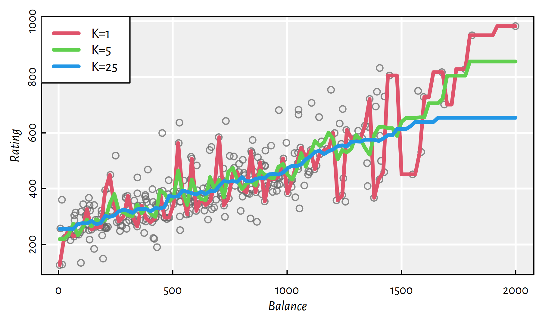

Figure 3.7: K-NN regression example

3.5.3 Further Reading

Recommended further reading: (Hastie et al. 2017: Section 13.3)