1 Simple Linear Regression
These lecture notes are distributed in the hope that they will be useful. Any bug reports are appreciated.
1.1 Machine Learning
1.1.1 What is Machine Learning?
An algorithm is a well-defined sequence of instructions that, for a given sequence of input arguments, yields some desired output.
In other words, it is a specific recipe for a function.
Developing algorithms is a tedious task.
In machine learning, we build and study computer algorithms that make predictions or decisions but which are not manually programmed.
Learning needs some material based upon which new knowledge is to be acquired.
In other words, we need data.
1.1.2 Main Types of Machine Learning Problems
Machine Learning Problems include, but are not limited to:
Supervised learning – for every input point (e.g., a photo) there is an associated desired output (e.g., whether it depicts a crosswalk or how many cars can be seen on it)
Unsupervised learning – inputs are unlabelled, the aim is to discover the underlying structure in the data (e.g., automatically group customers w.r.t. common behavioural patterns)
Semi-supervised learning – some inputs are labelled, the others are not (definitely a cheaper scenario)
Reinforcement learning – learn to act based on a feedback given after the actual decision was made (e.g., learn to play The Witcher 7 by testing different hypotheses what to do to survive as long as possible)
1.2 Supervised Learning
1.2.1 Formalism
Let \(\mathbf{X}=\{\mathfrak{X}_1,\dots,\mathfrak{X}_n\}\) be an input sample (“a database”) that consists of \(n\) objects.
Most often we assume that each object \(\mathfrak{X}_i\) is represented using \(p\) numbers for some \(p\).
We denote this fact as \(\mathfrak{X}_i\in \mathbb{R}^p\) (it is a \(p\)-dimensional real vector or a sequence of \(p\) numbers or a point in a \(p\)-dimensional real space or an element of a real \(p\)-space etc.).
If we have “complex” objects on input, we can always try representing them as feature vectors (e.g., come up with numeric attributes that best describe them in a task at hand).
Consider the following problems:
How would you represent a patient in a clinic?
How would you represent a car in an insurance company’s database?
How would you represent a student in an university?
Of course, our setting is abstract in the sense that there might be different realities hidden behind these symbols.
This is what maths is for – creating abstractions or models of complex entities/phenomena so that they can be much more easily manipulated or understood. This is very powerful – spend a moment contemplating how many real-world situations fit into our framework.
This also includes image/video data, e.g., a 1920×1080 pixel image can be “unwound” to a “flat” vector of length 2,073,600.
(*) There are some algorithms such as Multidimensional Scaling, Locally Linear Embedding, IsoMap etc. that can do that automagically.
In cases such as this we say that we deal with structured (tabular) data
– \(\mathbf{X}\) can be written as an (\(n\times p\))-matrix:
\[
\mathbf{X}=
\left[
\begin{array}{cccc}
x_{1,1} & x_{1,2} & \cdots & x_{1,p} \\
x_{2,1} & x_{2,2} & \cdots & x_{2,p} \\
\vdots & \vdots & \ddots & \vdots \\
x_{n,1} & x_{n,2} & \cdots & x_{n,p} \\
\end{array}
\right]
\]
Mathematically, we denote this as \(\mathbf{X}\in\mathbb{R}^{n\times p}\).
- Remark.
-
Structured data == think: Excel/Calc spreadsheets, SQL tables etc.
For an example, consider the famous Fisher’s Iris flower dataset,
see ?iris in R
and https://en.wikipedia.org/wiki/Iris_flower_data_set.
X <- iris[1:6, 1:4] # first 6 rows and 4 columns
X         # or: print(X)
## Sepal.Length Sepal.Width Petal.Length Petal.Width
## 1 5.1 3.5 1.4 0.2
## 2 4.9 3.0 1.4 0.2
## 3 4.7 3.2 1.3 0.2
## 4 4.6 3.1 1.5 0.2
## 5 5.0 3.6 1.4 0.2
## 6 5.4 3.9 1.7 0.4dim(X) # gives n and p## [1] 6 4dim(iris) # for the full dataset## [1] 150 5\(x_{i,j}\in\mathbb{R}\) represents the \(j\)-th feature of the \(i\)-th observation, \(j=1,\dots,p\), \(i=1,\dots,n\).
For instance:
X[3, 2] # 3rd row, 2nd column## [1] 3.2The third observation (data point, row in \(\mathbf{X}\)) consists of items \((x_{3,1}, \dots, x_{3,p})\) that can be extracted by calling:
X[3,]## Sepal.Length Sepal.Width Petal.Length Petal.Width
## 3 4.7 3.2 1.3 0.2as.numeric(X[3,]) # drops names## [1] 4.7 3.2 1.3 0.2length(X[3,])## [1] 4Moreover, the second feature/variable/column is comprised of \((x_{1,2}, x_{2,2}, \dots, x_{n,2})\):
X[,2]## [1] 3.5 3.0 3.2 3.1 3.6 3.9length(X[,2])## [1] 6We will sometimes use the following notation to emphasise that the \(\mathbf{X}\) matrix consists of \(n\) rows or \(p\) columns:
\[ \mathbf{X}=\left[ \begin{array}{c} \mathbf{x}_{1,\cdot} \\ \mathbf{x}_{2,\cdot} \\ \vdots\\ \mathbf{x}_{n,\cdot} \\ \end{array} \right] = \left[ \begin{array}{cccc} \mathbf{x}_{\cdot,1} & \mathbf{x}_{\cdot,2} & \cdots & \mathbf{x}_{\cdot,p} \\ \end{array} \right]. \]
Here, \(\mathbf{x}_{i,\cdot}\) is a row vector of length \(p\), i.e., a \((1\times p)\)-matrix:
\[ \mathbf{x}_{i,\cdot} = \left[ \begin{array}{cccc} x_{i,1} & x_{i,2} & \cdots & x_{i,p} \\ \end{array} \right]. \]
Moreover, \(\mathbf{x}_{\cdot,j}\) is a column vector of length \(n\), i.e., an \((n\times 1)\)-matrix:
\[ \mathbf{x}_{\cdot,j} = \left[ \begin{array}{cccc} x_{1,j} & x_{2,j} & \cdots & x_{n,j} \\ \end{array} \right]^T=\left[ \begin{array}{c} {x}_{1,j} \\ {x}_{2,j} \\ \vdots\\ {x}_{n,j} \\ \end{array} \right], \]
where \(\cdot^T\) denotes the transpose of a given matrix – think of this as a kind of rotation; it allows us to introduce a set of “vertically stacked” objects using a single inline formula.
1.2.2 Desired Outputs
In supervised learning, apart from the inputs we are also given the corresponding reference/desired outputs.
The aim of supervised learning is to try to create an “algorithm” that, given an input point, generates an output that is as close as possible to the desired one. The given data sample will be used to “train” this “model”.
Usually the reference outputs are encoded as individual numbers (scalars) or textual labels.
In other words, with each input \(\mathbf{x}_{i,\cdot}\) we associate the desired output \(y_i\):
# in iris, iris[, 5] gives the Ys
iris[sample(nrow(iris), 3), ]  # three random rows
## Sepal.Length Sepal.Width Petal.Length Petal.Width Species
## 14 4.3 3.0 1.1 0.1 setosa
## 50 5.0 3.3 1.4 0.2 setosa
## 118 7.7 3.8 6.7 2.2 virginicaHence, our dataset is \([\mathbf{X}\ \mathbf{y}]\) – each object is represented as a row vector \([\mathbf{x}_{i,\cdot}\ y_i]\), \(i=1,\dots,n\):
\[ [\mathbf{X}\ \mathbf{y}]= \left[ \begin{array}{ccccc} x_{1,1} & x_{1,2} & \cdots & x_{1,p} & y_1\\ x_{2,1} & x_{2,2} & \cdots & x_{2,p} & y_2\\ \vdots & \vdots & \ddots & \vdots & \vdots\\ x_{n,1} & x_{n,2} & \cdots & x_{n,p} & y_n\\ \end{array} \right], \]
where:
\[ \mathbf{y} = \left[ \begin{array}{cccc} y_{1} & y_{2} & \cdots & y_{n} \\ \end{array} \right]^T=\left[ \begin{array}{c} {y}_{1} \\ {y}_{2} \\ \vdots\\ {y}_{n} \\ \end{array} \right]. \]
1.2.3 Types of Supervised Learning Problems
Depending on the type of the elements in \(\mathbf{y}\) (the domain of \(\mathbf{y}\)), supervised learning problems are usually classified as:
regression – each \(y_i\) is a real number
e.g., \(y_i=\) future market stock price with \(\mathbf{x}_{i,\cdot}=\) prices from \(p\) previous days
classification – each \(y_i\) is a discrete label
e.g., \(y_i=\) healthy (0) or ill (1) with \(\mathbf{x}_{i,\cdot}=\) a patient’s health record
ordinal regression (a.k.a. ordinal classification) – each \(y_i\) is a rank
e.g., \(y_i=\) rating of a product on the scale 1–5 with \(\mathbf{x}_{i,\cdot}=\) ratings of \(p\) most similar products
Example Problems – Discussion:
Which of the following are instances of classification problems? Which of them are regression tasks?
What kind of data should you gather in order to tackle them?
- Detect email spam
- Predict a market stock price
- Predict the likeability of a new ad
- Assess credit risk
- Detect tumour tissues in medical images
- Predict time-to-recovery of cancer patients
- Recognise smiling faces on photographs
- Detect unattended luggage in airport security camera footage
- Turn on emergency braking to avoid a collision with pedestrians
A single dataset can become an instance of many different ML problems.
Examples – the wines dataset:
wines <- read.csv("datasets/winequality-all.csv", comment="#")
wines[1,]
## fixed.acidity volatile.acidity citric.acid residual.sugar chlorides
## 1 7.4 0.7 0 1.9 0.076
## free.sulfur.dioxide total.sulfur.dioxide density pH sulphates
## 1 11 34 0.9978 3.51 0.56
## alcohol response color
## 1 9.4 5 redalcohol is a numeric (quantitative) variable (see Figure 1.1 for a histogram depicting its empirical distribution):
summary(wines$alcohol) # continuous variable## Min. 1st Qu. Median Mean 3rd Qu. Max.
## 8.0 9.5 10.3 10.5 11.3 14.9hist(wines$alcohol, main="", col="white"); box()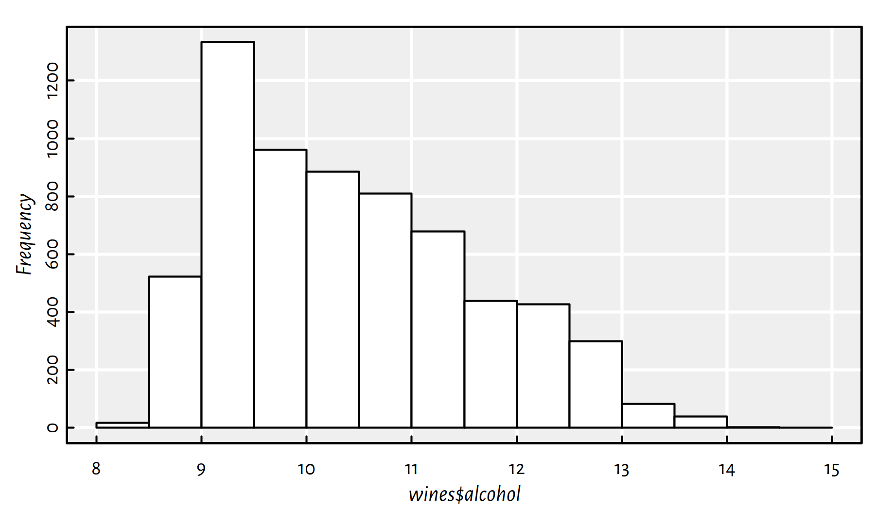
Figure 1.1: Quantitative (numeric) outputs lead to regression problems
color is a quantitative variable with two possible outcomes (see Figure 1.2 for a bar plot):
table(wines$color) # binary variable##
## red white
## 1599 4898barplot(table(wines$color), col="white", ylim=c(0, 6000))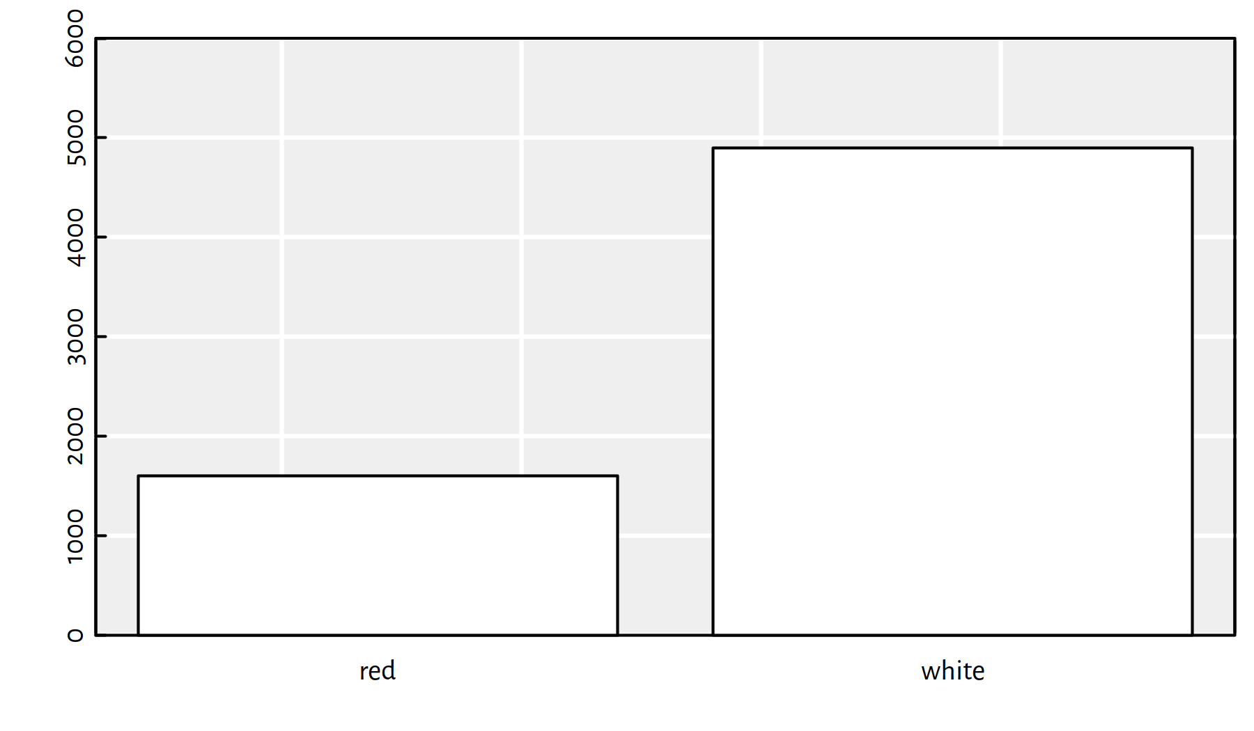
Figure 1.2: Quantitative outputs lead to classification tasks
Moreover, response is an ordinal variable, representing
a wine’s rating as assigned by a wine expert
(see Figure 1.3 for a barplot).
Note that although the ranks are represented with numbers,
we they are not continuous variables. Moreover,
these ranks are something more than just labels – they are linearly
ordered, we know what’s the smallest rank and whats the greatest one.
table(wines$response) # ordinal variable##
## 3 4 5 6 7 8 9
## 30 216 2138 2836 1079 193 5barplot(table(wines$response), col="white", ylim=c(0, 3000))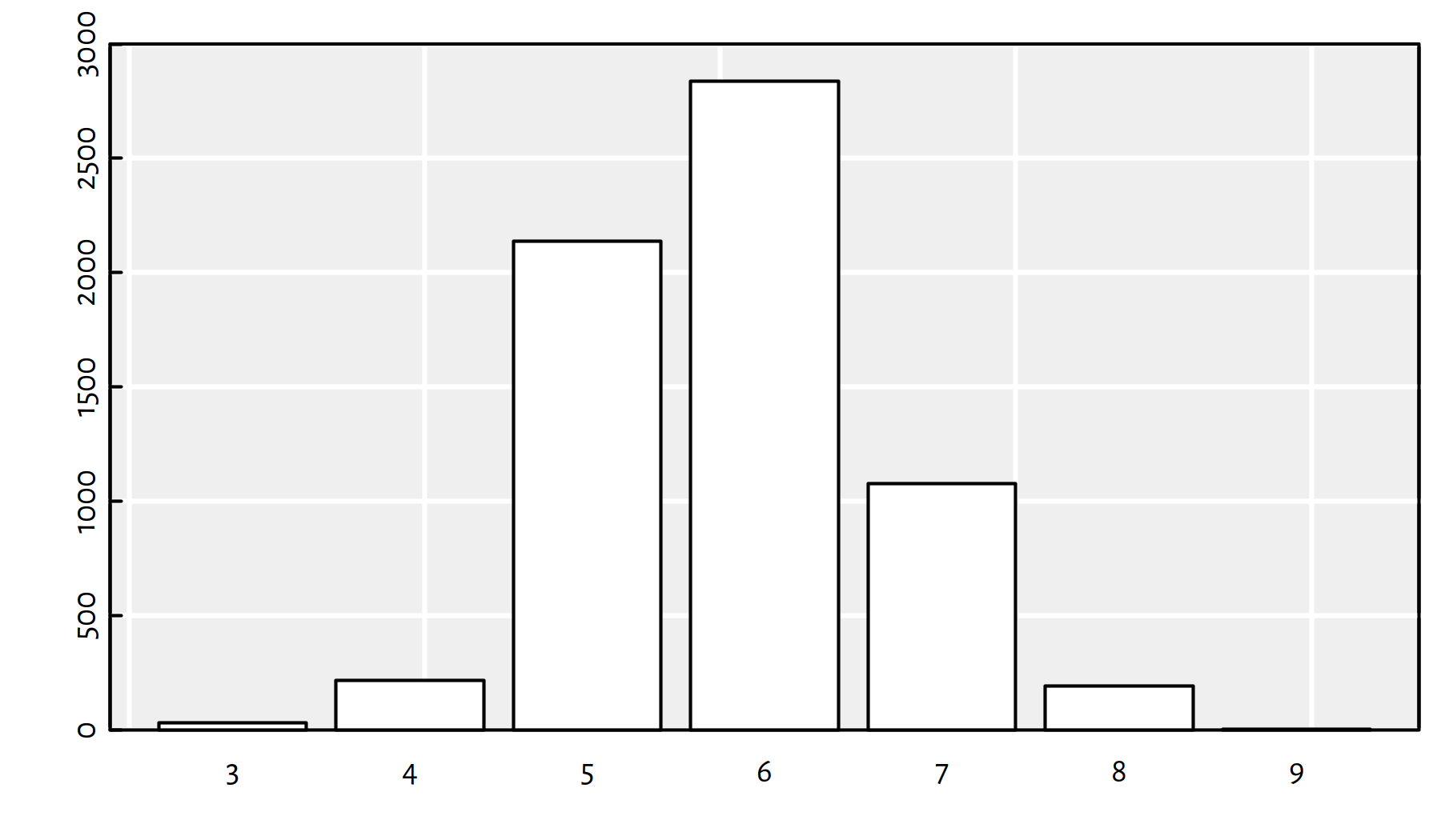
Figure 1.3: Ordinal variables constitute ordinal regression tasks
1.3 Simple Regression
1.3.1 Introduction
Simple regression is the easiest setting to start with – let’s assume \(p=1\), i.e., all inputs are 1-dimensional. Denote \(x_i=x_{i,1}\).
We will use it to build many intuitions, for example, it’ll be easy to illustrate all the concepts graphically.
library("ISLR") # Credit dataset
plot(Credit$Balance, Credit$Rating) # scatter plot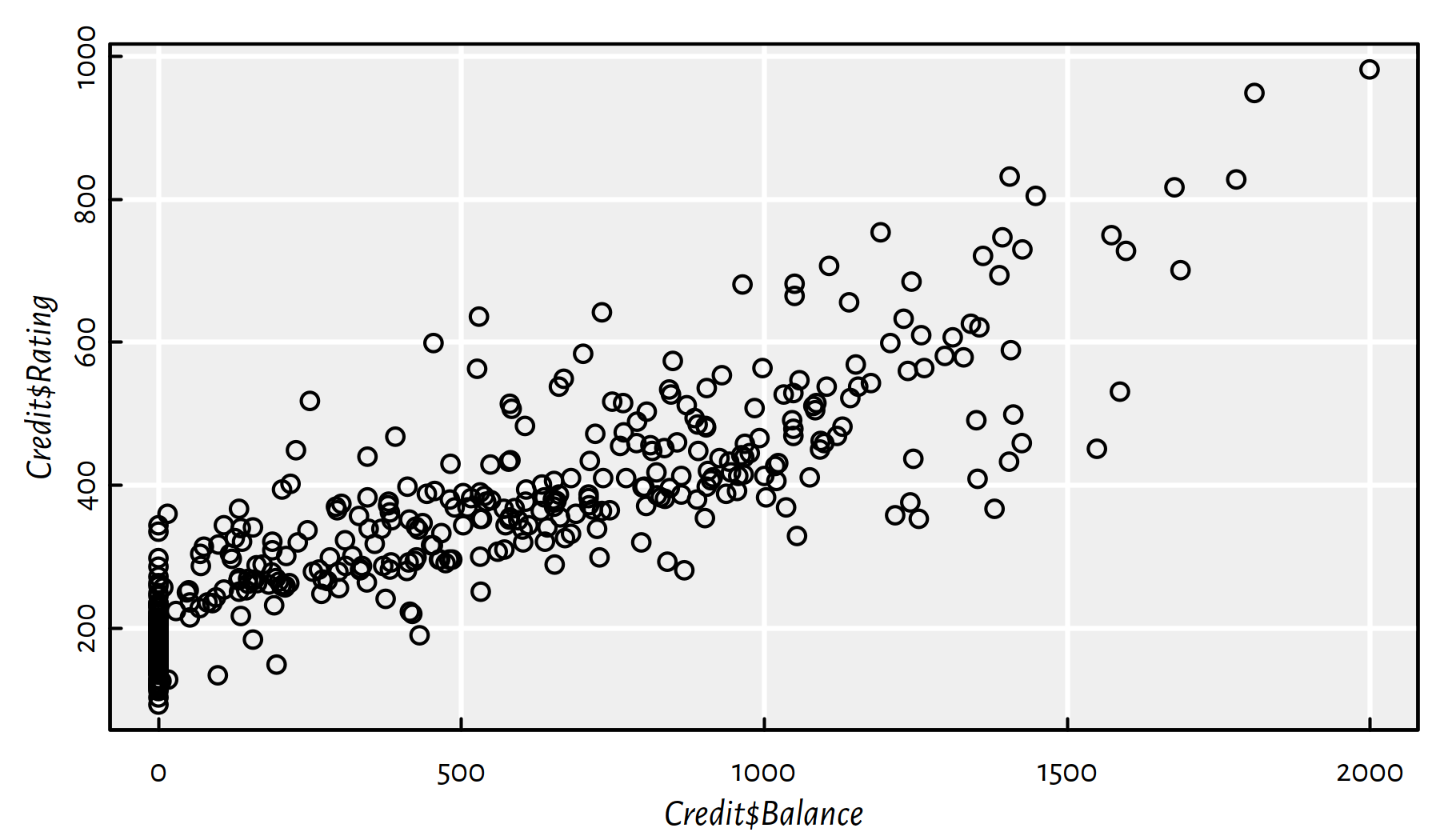
Figure 1.4: A scatter plot of Rating vs. Balance
In what follows we will be modelling the Credit Rating (\(Y\)) as a function of the average Credit Card Balance (\(X\)) in USD for customers with positive Balance only. It is because it is evident from Figure 1.4 that some customers with zero balance obtained a credit rating based on some external data source that we don’t have access to in our very setting.
X <- as.matrix(as.numeric(Credit$Balance[Credit$Balance>0]))
Y <- as.matrix(as.numeric(Credit$Rating[Credit$Balance>0]))
Figure 1.5 gives the updated scatter plot with the zero-balance clients “taken care of”.
plot(X, Y, xlab="X (Balance)", ylab="Y (Rating)")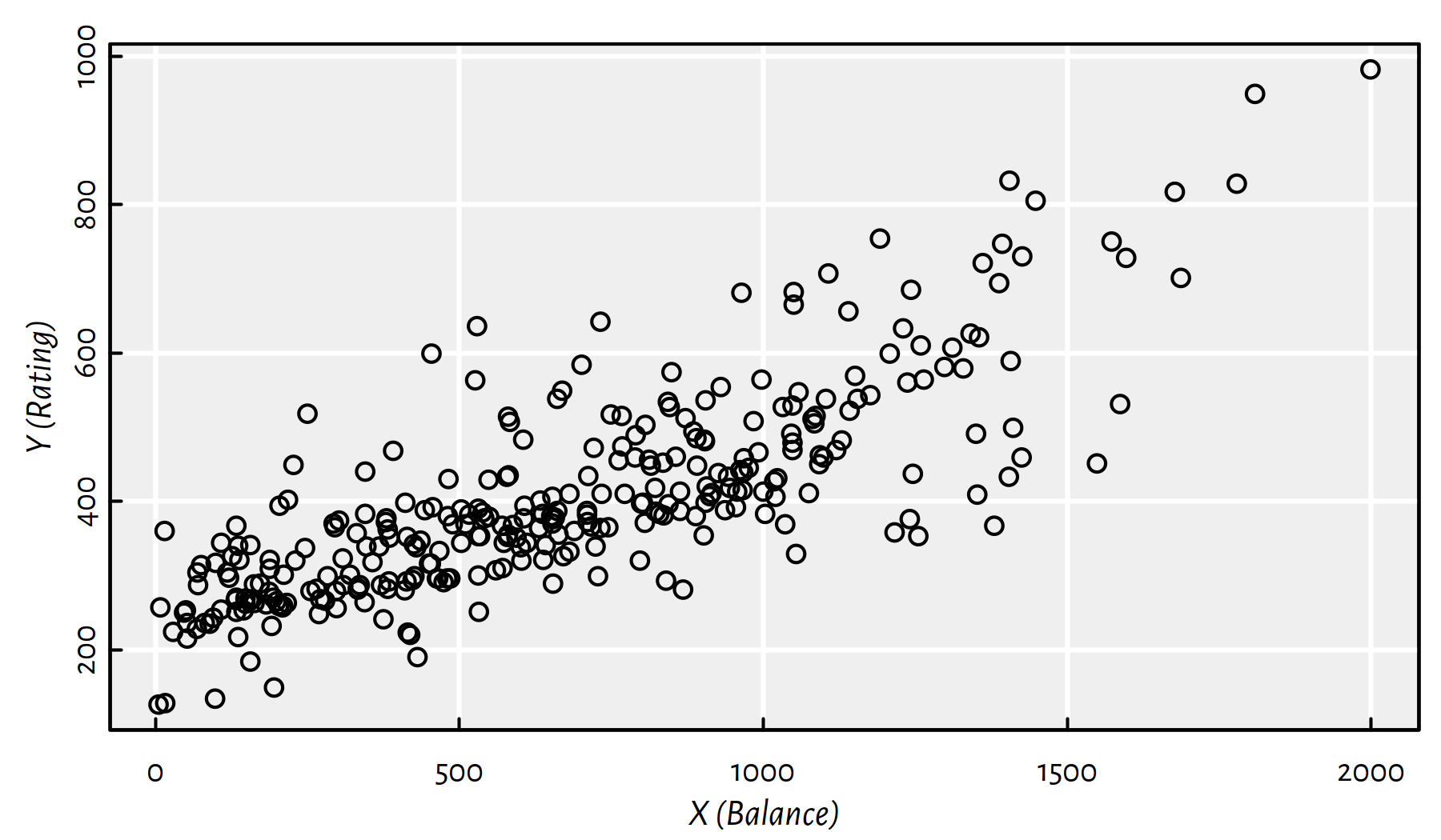
Figure 1.5: A scatter plot of Rating vs. Balance with clients of Balance=0 removed
Our aim is to construct a function \(f\) that models Rating as a function of Balance, \(f(X)=Y\).
We are equipped with \(n=310\) reference (observed) Ratings \(\mathbf{y}=[y_1\ \cdots\ y_n]^T\) for particular Balances \(\mathbf{x}=[x_1\ \cdots\ x_n]^T\).
Note the following naming conventions:
Variable types:
\(X\) – independent/explanatory/predictor variable
\(Y\) – dependent/response/predicted variable
Also note that:
\(Y\) – idealisation (any possible Rating)
\(\mathbf{y}=[y_1\ \cdots\ y_n]^T\) – values actually observed
The model will not be ideal, but it might be usable:
We will be able to predict the rating of any new client.
What should be the rating of a client with Balance of $1500?
What should be the rating of a client with Balance of $2500?
We will be able to describe (understand) this reality using a single mathematical formula so as to infer that there is an association between \(X\) and \(Y\)
Think of “data compression” and laws of physics, e.g., \(E=mc^2\).
(*) Mathematically, we will assume that there is some “true” function that models the data (true relationship between \(Y\) and \(X\)), but the observed outputs are subject to additive error: \[Y=f(X)+\varepsilon.\]
\(\varepsilon\) is a random term, classically we assume that errors are independent of each other, have expected value of \(0\) (there is no systematic error = unbiased) and that they follow a normal distribution.
(*) We denote this as \(\varepsilon\sim\mathcal{N}(0, \sigma)\) (read: random variable \(\varepsilon\) follows a normal distribution with expected value of \(0\) and standard deviation of \(\sigma\) for some \(\sigma\ge 0\)).
\(\sigma\) controls the amount of noise (and hence, uncertainty). Figure 1.6 gives the plot of the probability distribution function (PDFs, densities) of \(\mathcal{N}(0, \sigma)\) for different \(\sigma\)s:
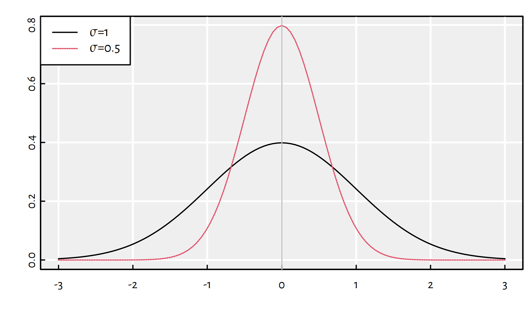
Figure 1.6: Probability density functions of normal distributions with different standard deviations \(\sigma\).
1.3.2 Search Space and Objective
There are many different functions that can be fitted into the observed \((\mathbf{x},\mathbf{y})\), compare Figure 1.7. Some of them are better than the other (with respect to different aspects, such as fit quality, simplicity etc.).
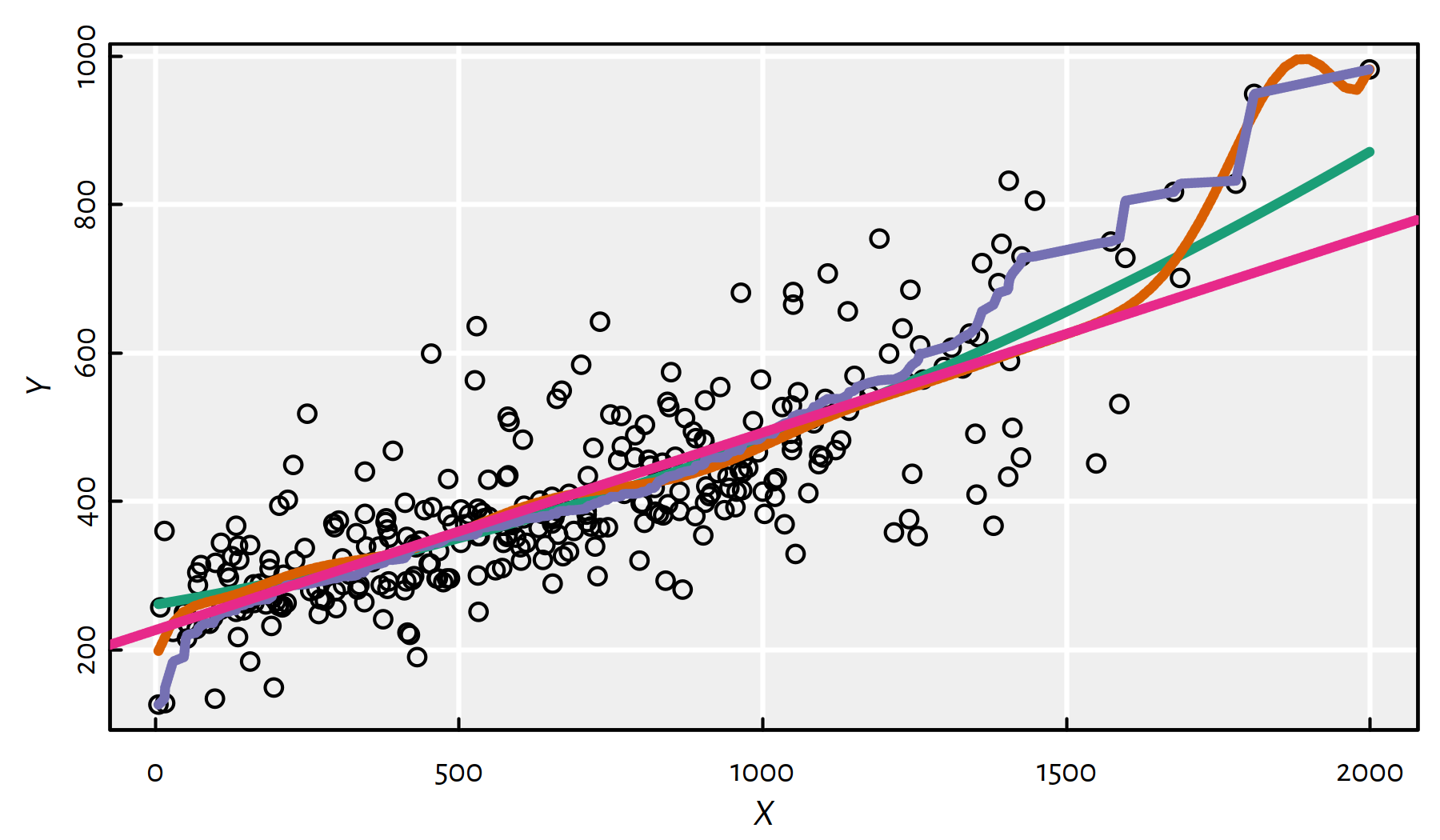
Figure 1.7: Different polynomial models fitted to data
Thus, we need a formal model selection criterion that could enable as to tackle the model fitting task on a computer.
Usually, we will be interested in a model that minimises appropriately aggregated residuals \(f(x_i)-y_i\), i.e., predicted outputs minus observed outputs, often denoted with \(\hat{y}_i-y_i\), for \(i=1,\dots,n\).
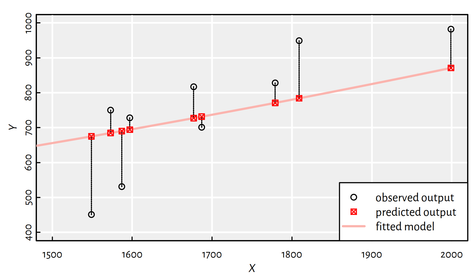
Figure 1.8: Residuals are defined as the differences between the predicted and observed outputs \(\hat{y}_i-y_i\)
In Figure 1.8, the residuals correspond to the lengths of the dashed line segments – they measure the discrepancy between the outputs generated by the model (what we get) and the true outputs (what we want).
Note that some sources define residuals as \(y_i-\hat{y}_i=y_i-f(x_i)\).
Top choice: sum of squared residuals: \[ \begin{array}{rl} \mathrm{SSR}(f|\mathbf{x},\mathbf{y}) & = \left( f(x_1)-y_1 \right)^2 + \dots + \left( f(x_n)-y_n \right)^2 \\ & = \displaystyle\sum_{i=1}^n \left( f(x_i)-y_i \right)^2 \end{array} \]
- Remark.
-
Read “\(\sum_{i=1}^n z_i\)” as “the sum of \(z_i\) for \(i\) from \(1\) to \(n\)”; this is just a shorthand for \(z_1+z_2+\dots+z_n\).
- Remark.
-
The notation \(\mathrm{SSR}(f|\mathbf{x},\mathbf{y})\) means that it is the error measure corresponding to the model \((f)\) given our data.
We could’ve denoted it with \(\mathrm{SSR}_{\mathbf{x},\mathbf{y}}(f)\) or even \(\mathrm{SSR}(f)\) to emphasise that \(\mathbf{x},\mathbf{y}\) are just fixed values and we are not interested in changing them at all (they are “global variables”).
We enjoy SSR because (amongst others):
larger errors are penalised much more than smaller ones
(this can be considered a drawback as well)
(**) statistically speaking, this has a clear underlying interpretation
(assuming errors are normally distributed, finding a model minimising the SSR is equivalent to maximum likelihood estimation)
the models minimising the SSR can often be found easily
(corresponding optimisation tasks have an analytic solution – studied already by Gauss in the late 18th century)
(**) Other choices:
- regularised SSR, e.g., lasso or ridge regression (in the case of multiple input variables)
- sum or median of absolute values (robust regression)
Fitting a model to data can be written as an optimisation problem:
\[ \min_{f\in\mathcal{F}} \mathrm{SSR}(f|\mathbf{x},\mathbf{y}), \]
i.e., find \(f\) minimising the SSR (seek “best” \(f\))
amongst the set of admissible models \(\mathcal{F}\).
Example \(\mathcal{F}\)s:
\(\mathcal{F}=\{\text{All possible functions of one variable}\}\) – if there are no repeated \(x_i\)’s, this corresponds to data interpolation; note that there are many functions that give SSR of \(0\).
\(\mathcal{F}=\{ x\mapsto x^2, x\mapsto \cos(x), x\mapsto \exp(2x+7)-9 \}\) – obviously an ad-hoc choice but you can easily choose the best amongst the 3 by computing 3 sums of squares.
\(\mathcal{F}=\{ x\mapsto a+bx\}\) – the space of linear functions of one variable
etc.
(e.g., \(x\mapsto x^2\) is read “\(x\) maps to \(x^2\)” and is an elegant way to define an inline function \(f\) such that \(f(x)=x^2\))
1.4 Simple Linear Regression
1.4.1 Introduction
If the family of admissible models \(\mathcal{F}\) consists only of all linear functions of one variable, we deal with a simple linear regression.
Our problem becomes:
\[ \min_{a,b\in\mathbb{R}} \sum_{i=1}^n \left( a+bx_i-y_i \right)^2 \]
In other words, we seek best fitting line in terms of the squared residuals.
This is the method of least squares.
This is particularly nice, because our search space is just \(\mathbb{R}^2\) – easy to handle both analytically and numerically.
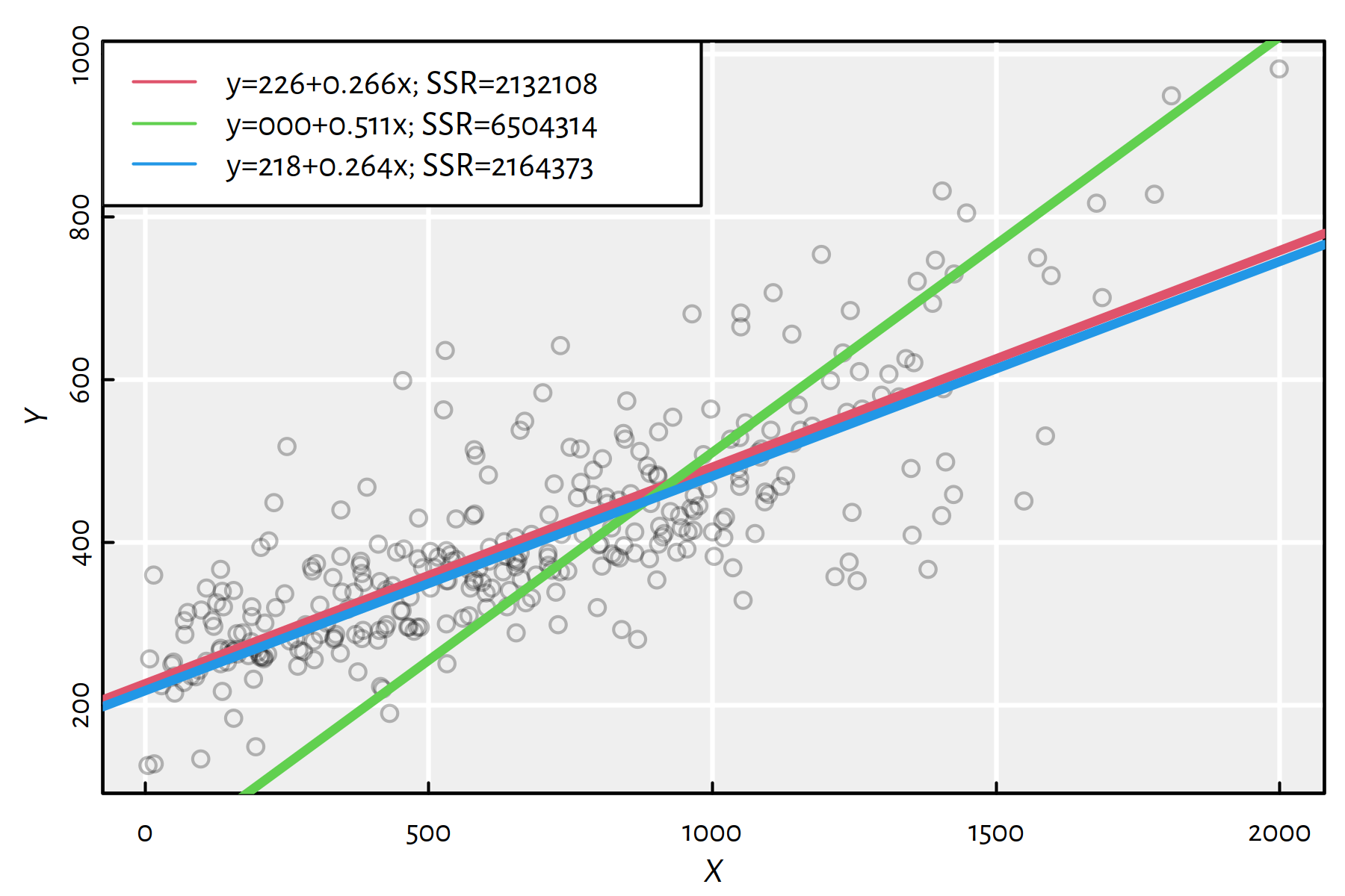
Figure 1.9: Three simple linear models together with the corresponding SSRs
Which of the lines in Figure 1.9 is the least squares solution?
1.4.2 Solution in R
Let’s fit the linear model minimising the SSR in R.
The lm() function (linear models) has a convenient formula-based interface.
f <- lm(Y~X)In R, the expression “Y~X” denotes a formula, which we read as:
variable Y is a function of X.
Note that the dependent variable is on the left side of the formula.
Here, X and Y are two R numeric vectors of identical lengths.
Let’s print the fitted model:
print(f)##
## Call:
## lm(formula = Y ~ X)
##
## Coefficients:
## (Intercept) X
## 226.471 0.266Hence, the fitted model is: \[ Y = f(X) = 226.47114+0.26615 X \qquad (+ \varepsilon) \]
Coefficient \(a\) (intercept):
f$coefficient[1]## (Intercept)
## 226.47Coefficient \(b\) (slope):
f$coefficient[2]## X
## 0.26615Plotting, see Figure 1.10:
plot(X, Y, col="#000000aa")
abline(f, col=2, lwd=3)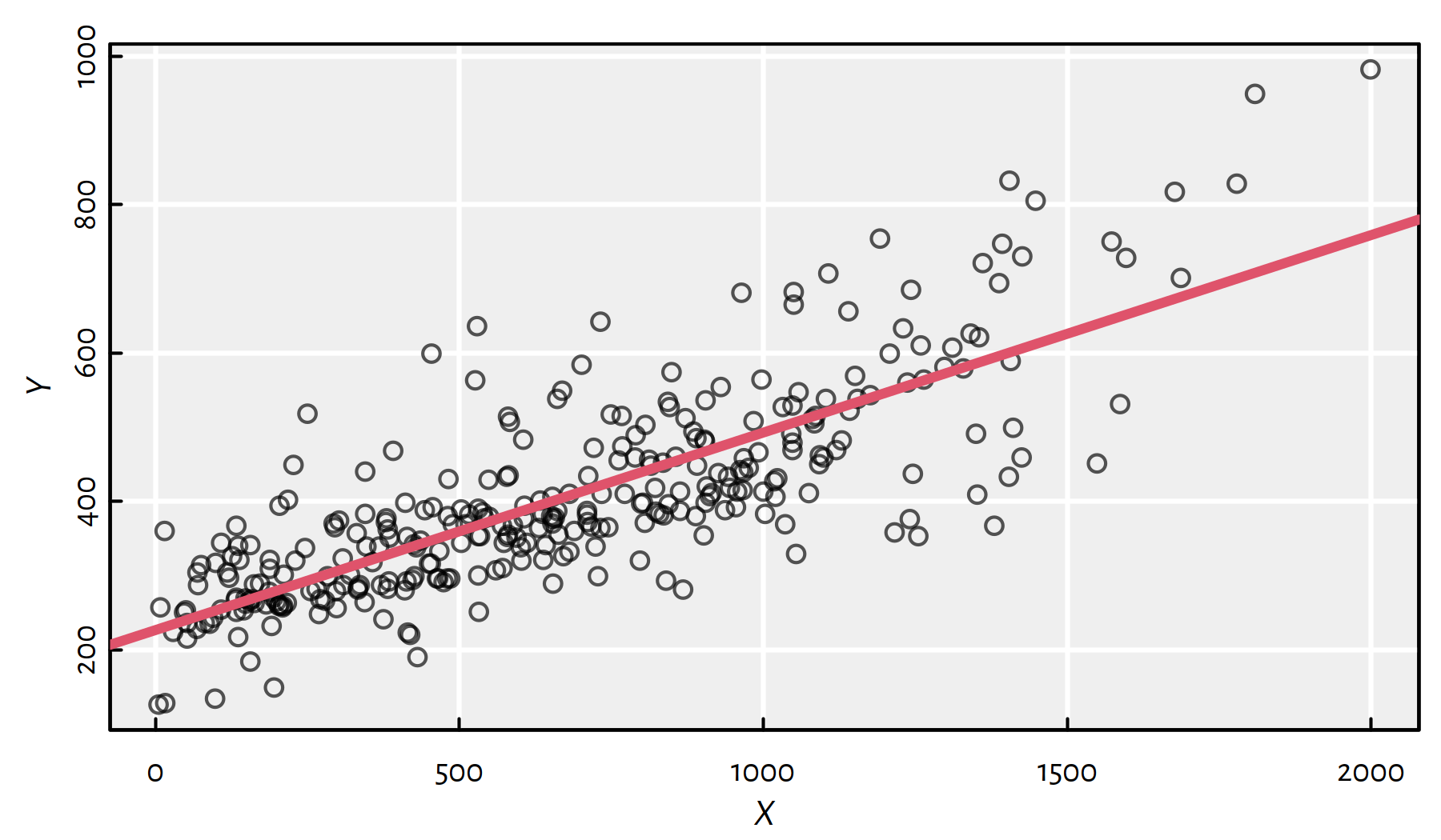
Figure 1.10: Fitted regression line
SSR:
sum(f$residuals^2)## [1] 2132108sum((f$coefficient[1]+f$coefficient[2]*X-Y)^2) # equivalent## [1] 2132108We can predict the model’s output for yet-unobserved inputs by writing:
X_new <- c(1500, 2000, 2500) # example inputs
f$coefficient[1] + f$coefficient[2]*X_new
## [1] 625.69 758.76 891.84Note that linear models can also be fitted based on formulas that refer to a data frame’s columns. For example, let us wrap both \(\mathbf{x}\) and \(\mathbf{y}\) inside a data frame:
XY <- data.frame(Balance=X, Rating=Y)
head(XY, 3)
## Balance Rating
## 1 333 283
## 2 903 483
## 3 580 514By writing:
f <- lm(Rating~Balance, data=XY)now Balance and Rating refer to column names in the XY data frame,
and not the objects in R’s “workspace”.
Based on the above, we can make a prediction
using the predict() function”
X_new <- data.frame(Balance=c(1500, 2000, 2500))
predict(f, X_new)
## 1 2 3
## 625.69 758.76 891.84Interestingly:
predict(f, data.frame(Balance=c(5000)))## 1
## 1557.2This is more than the highest possible rating – we have extrapolated way beyond the observable data range.
Note that our \(Y=a+bX\) model is interpretable and well-behaving (not all machine learning models will have this feature, think: deep neural networks, which we rather conceive as black boxes):
we know that by increasing \(X\) by a small amount, \(Y\) will also increase (positive correlation),
the model is continuous – small change in \(X\) doesn’t yield any drastic change in \(Y\),
we know what will happen if we increase or decrease \(X\) by, say, \(100\),
the function is invertible – if we want Rating of \(500\), we can compute the associated preferred Balance that should yield it (provided that the model is valid).
1.4.3 Analytic Solution
It may be shown (which we actually do below) that the solution is:
\[ \left\{ \begin{array}{rl} b = & \dfrac{ n \displaystyle\sum_{i=1}^n x_i y_i - \displaystyle\sum_{i=1}^n y_i \displaystyle\sum_{i=1}^n x_i }{ n \displaystyle\sum_{i=1}^n x_i x_i - \displaystyle\sum_{i=1}^n x_i\displaystyle\sum_{i=1}^n x_i }\\ a = & \dfrac{1}{n}\displaystyle\sum_{i=1}^n y_i - b \dfrac{1}{n} \displaystyle\sum_{i=1}^n x_i \\ \end{array} \right. \]
Which can be implemented in R as follows:
n <- length(X)
b <- (n*sum(X*Y)-sum(X)*sum(Y))/(n*sum(X*X)-sum(X)^2)
a <- mean(Y)-b*mean(X)
c(a, b) # the same as f$coefficients
## [1] 226.47114 0.266151.4.4 Derivation of the Solution (**)
- Remark.
-
You can safely skip this part if you are yet to know how to search for a minimum of a function of many variables and what are partial derivatives.
Denote with:
\[ E(a,b)=\mathrm{SSR}(x\mapsto a+bx|\mathbf{x},\mathbf{y}) =\sum_{i=1}^n \left( a+bx_i - y_i \right) ^2. \]
We seek the minimum of \(E\) w.r.t. both \(a,b\).
- Theorem.
-
If \(E\) has a (local) minimum at \((a^*,b^*)\), then its partial derivatives vanish therein, i.e., \(\partial E/\partial a(a^*, b^*) = 0\) and \(\partial E/\partial b(a^*, b^*)=0\).
We have:
\[ E(a,b) = \displaystyle\sum_{i=1}^n \left( a+bx_i - y_i \right) ^2. \]
We need to compute the partial derivatives \(\partial E/\partial a\) (derivative of \(E\) w.r.t. variable \(a\) – all other terms treated as constants) and \(\partial E/\partial b\) (w.r.t. \(b\)).
Useful rules – derivatives w.r.t. \(a\) (denote \(f'(a)=(f(a))'\)):
- \((f(a)+g(a))'=f'(a)+g'(a)\) (derivative of sum is sum of derivatives)
- \((f(a) g(a))' = f'(a)g(a) + f(a)g'(a)\) (derivative of product)
- \((f(g(a)))' = f'(g(a)) g'(a)\) (chain rule)
- \((c)' = 0\) for any constant \(c\) (expression not involving \(a\))
- \((a^p)' = pa^{p-1}\) for any \(p\)
- in particular: \((c a^2+d)'=2ca\), \((ca)'=c\), \(((ca+d)^2)'=2(ca+d)c\) (application of the above rules)
We seek \(a,b\) such that \(\frac{\partial E}{\partial a}(a,b) = 0\) and \(\frac{\partial E}{\partial b}(a,b)=0\).
\[ \left\{ \begin{array}{rl} \frac{\partial E}{\partial a}(a,b)=&2\displaystyle\sum_{i=1}^n \left( a+bx_i - y_i \right) = 0\\ \frac{\partial E}{\partial b}(a,b)=&2\displaystyle\sum_{i=1}^n \left( a+bx_i - y_i \right) x_i = 0 \\ \end{array} \right. \]
This is a system of 2 linear equations. Easy.
Rearranging like back in the school days:
\[ \left\{ \begin{array}{rl} b \displaystyle\sum_{i=1}^n x_i+ a n = & \displaystyle\sum_{i=1}^n y_i \\ b \displaystyle\sum_{i=1}^n x_i x_i + a \displaystyle\sum_{i=1}^n x_i = & \displaystyle\sum_{i=1}^n x_i y_i \\ \end{array} \right. \]
It is left as an exercise to show that the solution is:
\[ \left\{ \begin{array}{rl} b^* = & \dfrac{ n \displaystyle\sum_{i=1}^n x_i y_i - \displaystyle\sum_{i=1}^n y_i \displaystyle\sum_{i=1}^n x_i }{ n \displaystyle\sum_{i=1}^n x_i x_i - \displaystyle\sum_{i=1}^n x_i\displaystyle\sum_{i=1}^n x_i }\\ a^* = & \dfrac{1}{n}\displaystyle\sum_{i=1}^n y_i - b^* \dfrac{1}{n} \displaystyle\sum_{i=1}^n x_i \\ \end{array} \right. \]
(we should additionally perform the second derivative test to assure that this is the minimum of \(E\) – which is exactly the case though)
(**) In the next chapter, we will introduce the notion of Pearson’s
linear coefficient, \(r\) (see cor() in R). It might be shown that
\(a\) and \(b\) can also be rewritten as:
(b <- cor(X,Y)*sd(Y)/sd(X))## [,1]
## [1,] 0.26615(a <- mean(Y)-b*mean(X))## [,1]
## [1,] 226.471.5 Exercises in R
1.5.1 The Anscombe Quartet
Here is a famous illustrative example proposed by the statistician Francis Anscombe in the early 1970s.
print(anscombe) # `anscombe` is a built-in object## x1 x2 x3 x4 y1 y2 y3 y4
## 1 10 10 10 8 8.04 9.14 7.46 6.58
## 2 8 8 8 8 6.95 8.14 6.77 5.76
## 3 13 13 13 8 7.58 8.74 12.74 7.71
## 4 9 9 9 8 8.81 8.77 7.11 8.84
## 5 11 11 11 8 8.33 9.26 7.81 8.47
## 6 14 14 14 8 9.96 8.10 8.84 7.04
## 7 6 6 6 8 7.24 6.13 6.08 5.25
## 8 4 4 4 19 4.26 3.10 5.39 12.50
## 9 12 12 12 8 10.84 9.13 8.15 5.56
## 10 7 7 7 8 4.82 7.26 6.42 7.91
## 11 5 5 5 8 5.68 4.74 5.73 6.89What we see above is a single data frame
that encodes four separate datasets:
anscombe$x1 and anscombe$y1 define the first pair of variables,
anscombe$x2 and anscombe$y2 define the second pair and so forth.
Split the above data (manually) into four data frames
ans1, …, ans4 with columns x and y.
For example, ans1 should look like:
print(ans1)## x y
## 1 10 8.04
## 2 8 6.95
## 3 13 7.58
## 4 9 8.81
## 5 11 8.33
## 6 14 9.96
## 7 6 7.24
## 8 4 4.26
## 9 12 10.84
## 10 7 4.82
## 11 5 5.68Click here for a solution.
ans1 <- data.frame(x=anscombe$x1, y=anscombe$y1)
ans2 <- data.frame(x=anscombe$x2, y=anscombe$y2)
ans3 <- data.frame(x=anscombe$x3, y=anscombe$y3)
ans4 <- data.frame(x=anscombe$x4, y=anscombe$y4)
print(ans1)Compute the mean of each x and y variable.
Click here for a solution.
mean(ans1$x) # individual column## [1] 9mean(ans1$y) # individual column## [1] 7.5009sapply(ans2, mean) # all columns in ans2## x y
## 9.0000 7.5009sapply(anscombe, mean) # all columns in the full anscombe dataset## x1 x2 x3 x4 y1 y2 y3 y4
## 9.0000 9.0000 9.0000 9.0000 7.5009 7.5009 7.5000 7.5009Comment: This is really interesting, all the means of x columns
as well as the means of ys are almost identical.
Compute the standard deviation of each x and y variable.
Click here for a solution.
The solution is similar to the previous one, just replace mean with sd.
Here, to learn something new, we will use the knitr::kable() function
that pretty-prints a given matrix or data frame:
results <- sapply(anscombe, sd)
knitr::kable(results, col.names="standard deviation")| standard deviation | |
|---|---|
| x1 | 3.3166 |
| x2 | 3.3166 |
| x3 | 3.3166 |
| x4 | 3.3166 |
| y1 | 2.0316 |
| y2 | 2.0317 |
| y3 | 2.0304 |
| y4 | 2.0306 |
Comment: This is even more interesting, because the numbers agree up to 2 decimal digits.
Fit a simple linear regression model for each data set.
Draw the scatter plots again (plot())
and add the regression lines (lines() or abline()).
Click here for a solution.
To recall, this can be done with the lm() function
explained in Lecture 2.
At this point we should already have become lazy – the tasks are very repetitious. Let’s automate them by writing a single function that does all the above for any data set:
fit_models <- function(ans) {
    # ans is a data frame with columns x and y
    f <- lm(y~x, data=ans) # fit linear model
    print(f$coefficients) # estimated coefficients
    plot(ans$x, ans$y) # scatter plot
    abline(f, col="red") # regression line
    return(f)
}
Now we can apply it on the four particular examples.
par(mfrow=c(2, 2)) # four plots on 1 figure (2x2 grid)
f1 <- fit_models(ans1)
## (Intercept) x
## 3.00009 0.50009f2 <- fit_models(ans2)## (Intercept) x
## 3.0009 0.5000f3 <- fit_models(ans3)## (Intercept) x
## 3.00245 0.49973f4 <- fit_models(ans4)## (Intercept) x
## 3.00173 0.49991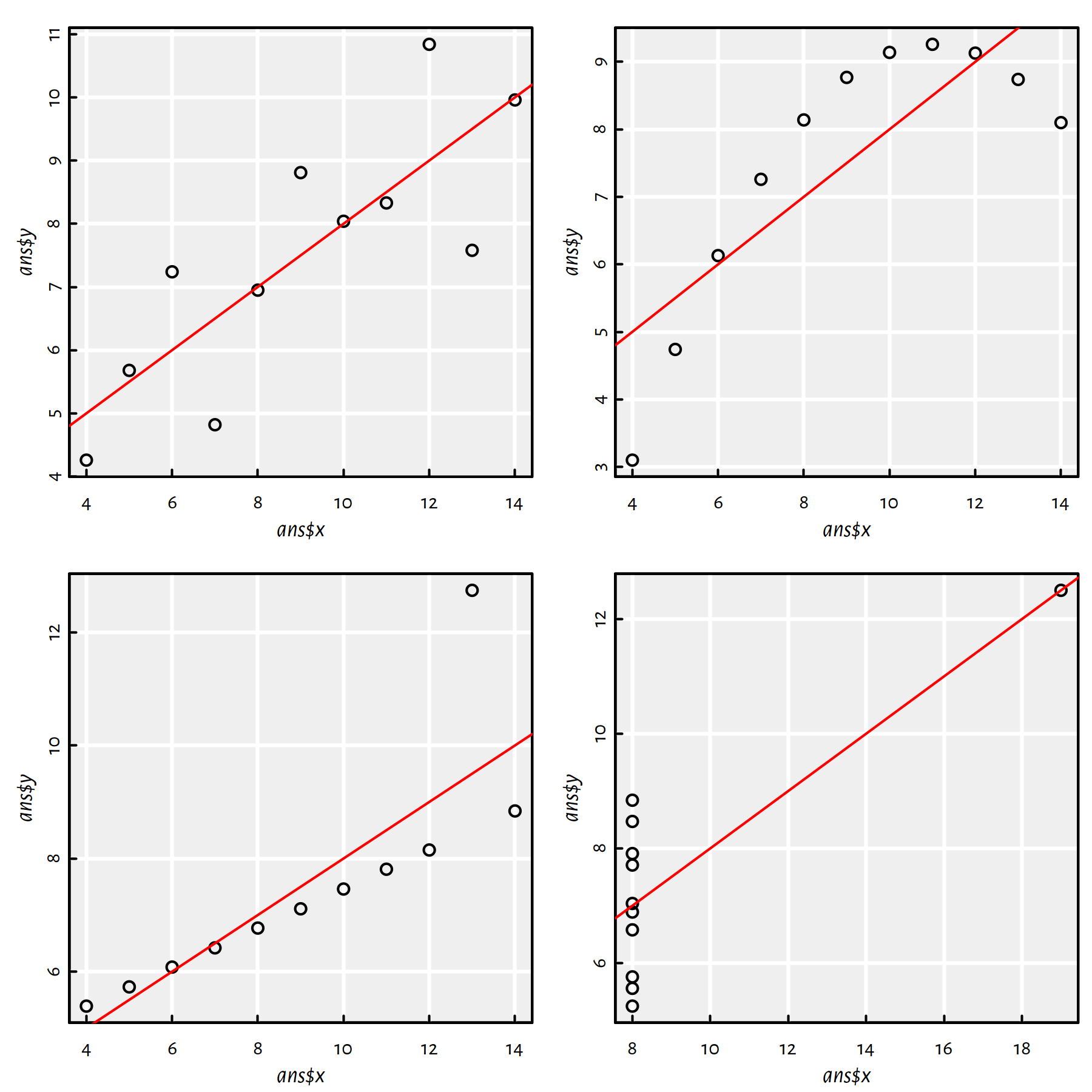
Figure 1.11: Fitted regression lines for the Anscombe quartet
Comment: All the estimated models are virtually the same, the regression lines are \(y=0.5x+3\), compare Figure 1.11.
Create scatter plots of the residuals (predicted \(\hat{y}_i\) minus true \(y_i\)) as a function of the predicted \(\hat{y}_i=f(x_i)\) for every \(i=1,\dots,11\).
Click here for a solution.
To recall, the model predictions can be generated by (amongst others)
calling the predict() function.
y_pred1 <- f1$fitted.values # predict(f1, ans1)
y_pred2 <- f2$fitted.values # predict(f2, ans2)
y_pred3 <- f3$fitted.values # predict(f3, ans3)
y_pred4 <- f4$fitted.values # predict(f4, ans4)
Plots of residuals as a function of the predicted (fitted) values are given in Figure 1.12.
par(mfrow=c(2, 2)) # four plots on 1 figure (2x2 grid)
plot(y_pred1, y_pred1-ans1$y)
plot(y_pred2, y_pred2-ans2$y)
plot(y_pred3, y_pred3-ans3$y)
plot(y_pred4, y_pred4-ans4$y)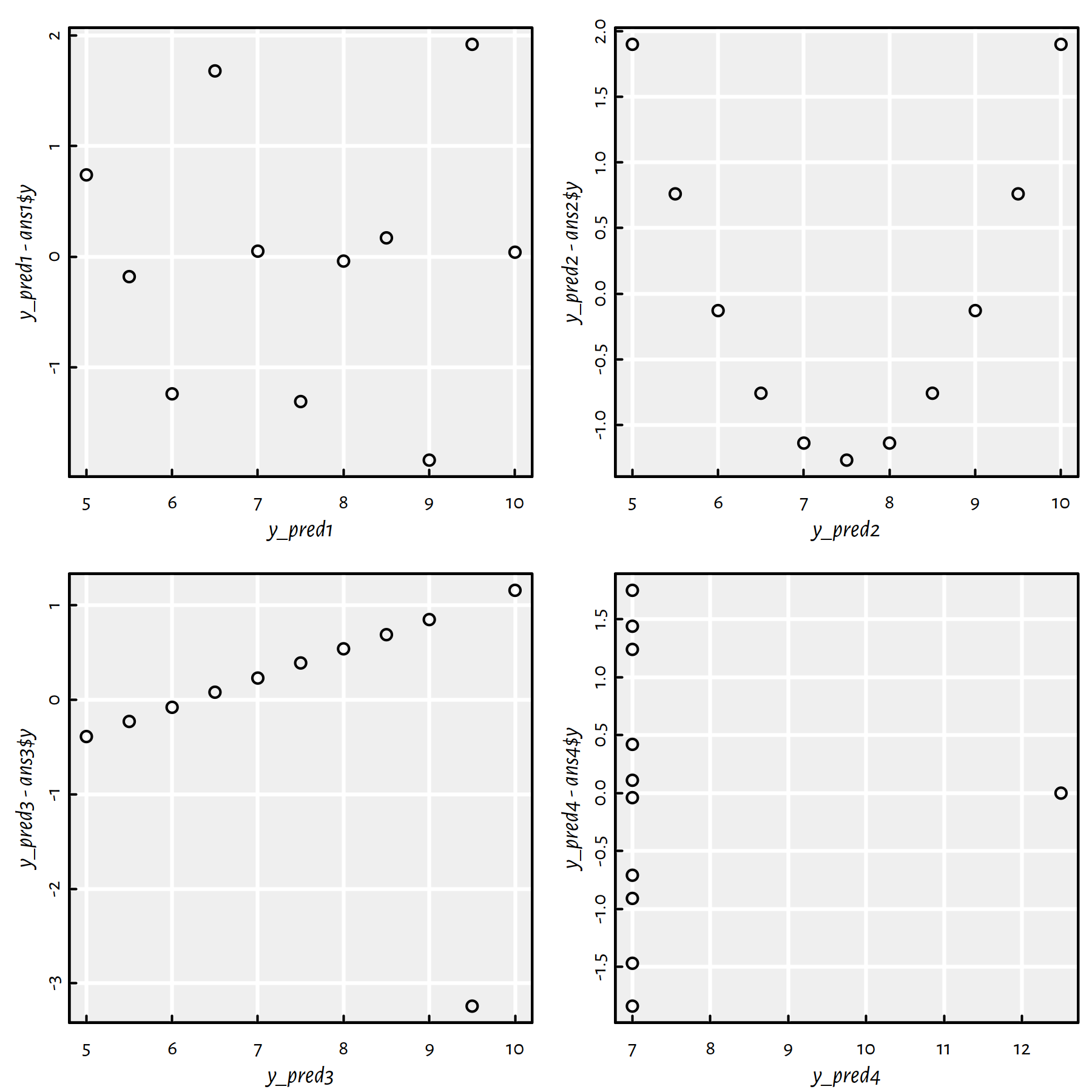
Figure 1.12: Residuals vs. fitted values for the regression lines fitted to the Anscombe quartet
Comment: Ideally, the residuals shouldn’t be correlated with the predicted values – they should “oscillate” randomly around 0. This is only the case of the first dataset. All the other cases are “alarming” in the sense that they suggest that the obtained models are “suspicious” (perhaps data cleansing is needed or a linear model is not at all appropriate).
Draw conclusions (in your own words).
Click here for a solution.
We’re being taught a lesson here: don’t perform data analysis tasks automatically, don’t look at bare numbers only, visualise your data first!
Read more about Anscombe’s quartet at https://en.wikipedia.org/wiki/Anscombe%27s_quartet
1.6 Outro
1.6.1 Remarks
In supervised learning, with each input point, there’s an associated reference output value.
Learning a model = constructing a function that approximates (minimising some error measure) the given data.
Regression = the output variable \(Y\) is continuous.
We studied linear models with a single independent variable based on the least squares (SSR) fit.
In the next part we will extend this setting to the case of many variables, i.e., \(p>1\), called multiple regression.
1.6.2 Further Reading
Recommended further reading: (James et al. 2017: Chapters 1, 2 and 3)
Other: (Hastie et al. 2017: Chapter 1, Sections 3.2 and 3.3)