5 Shallow and Deep Neural Networks (*)
These lecture notes are distributed in the hope that they will be useful. Any bug reports are appreciated.
5.1 Introduction
5.1.1 Binary Logistic Regression: Recap
Let \(\mathbf{X}\in\mathbb{R}^{n\times p}\) be an input matrix that consists of \(n\) points in a \(p\)-dimensional space.
\[ \mathbf{X}= \left[ \begin{array}{cccc} x_{1,1} & x_{1,2} & \cdots & x_{1,p} \\ x_{2,1} & x_{2,2} & \cdots & x_{2,p} \\ \vdots & \vdots & \ddots & \vdots \\ x_{n,1} & x_{n,2} & \cdots & x_{n,p} \\ \end{array} \right] \]
In other words, we have a database on \(n\) objects. Each object is described by means of \(p\) numerical features.
With each input \(\mathbf{x}_{i,\cdot}\) we associate the desired output \(y_i\) which is a categorical label – hence we will be dealing with classification tasks again.
To recall, in binary logistic regression we model the probabilities that a given input belongs to either of the two classes:
\[ \begin{array}{lr} \Pr(Y=1|\mathbf{X},\boldsymbol\beta)=& \phi(\beta_0 + \beta_1 X_1 + \dots + \beta_p X_p)\\ \Pr(Y=0|\mathbf{X},\boldsymbol\beta)=& 1-\phi(\beta_0 + \beta_1 X_1 + \dots + \beta_p X_p)\\ \end{array} \] where \(\phi(t) = \frac{1}{1+e^{-t}}=\frac{e^t}{1+e^t}\) is the logistic sigmoid function.
It holds: \[ \begin{array}{ll} \Pr(Y=1|\mathbf{X},\boldsymbol\beta)=&\displaystyle\frac{1}{1+e^{-(\beta_0 + \beta_1 X_1 + \dots + \beta_p X_p)}},\\ \Pr(Y=0|\mathbf{X},\boldsymbol\beta)=& \displaystyle\frac{1}{1+e^{+(\beta_0 + \beta_1 X_1 + \dots + \beta_p X_p)}}=\displaystyle\frac{e^{-(\beta_0 + \beta_1 X_1 + \dots + \beta_p X_p)}}{1+e^{-(\beta_0 + \beta_1 X_1 + \dots + \beta_p X_p)}}.\\ \end{array} \]
The fitting of the model was performed by minimising the cross-entropy (log-loss): \[ \min_{\boldsymbol\beta\in\mathbb{R}^{p+1}} -\frac{1}{n} \sum_{i=1}^n \Bigg(y_i\log \hat{y}_i + (1-y_i)\log (1-\hat{y}_i)\Bigg). \] where \(\hat{y}_i=\Pr(Y=1|\mathbf{x}_{i,\cdot},\boldsymbol\beta)\).
This is equivalent to: \[ \min_{\boldsymbol\beta\in\mathbb{R}^{p+1}} -\frac{1}{n} \sum_{i=1}^n \Bigg(y_i\log \Pr(Y=1|\mathbf{x}_{i,\cdot},\boldsymbol\beta) + (1-y_i)\log \Pr(Y=0|\mathbf{x}_{i,\cdot},\boldsymbol\beta)\Bigg). \]
Note that for each \(i\), either the left or the right term (in the bracketed expression) vanishes.
Hence, we may also write the above as: \[ \min_{\boldsymbol\beta\in\mathbb{R}^{p+1}} -\frac{1}{n} \sum_{i=1}^n \log \Pr(Y=y_i|\mathbf{x}_{i,\cdot},\boldsymbol\beta). \]
In this chapter we will generalise the binary logistic regression model:
First we will consider the case of many classes (multiclass classification). This will lead to the multinomial logistic regression model.
Then we will note that the multinomial logistic regression is a special case of a feed-forward neural network.
5.1.2 Data
We will study the famous classic – the MNIST image classification dataset (Modified National Institute of Standards and Technology database), see http://yann.lecun.com/exdb/mnist/
It consists of 28×28 pixel images of handwritten digits:
train: 60,000 training images,t10k: 10,000 testing images.
A few image instances from each class are depicted in Figure 5.1.
## Loaded Tensorflow version 2.9.1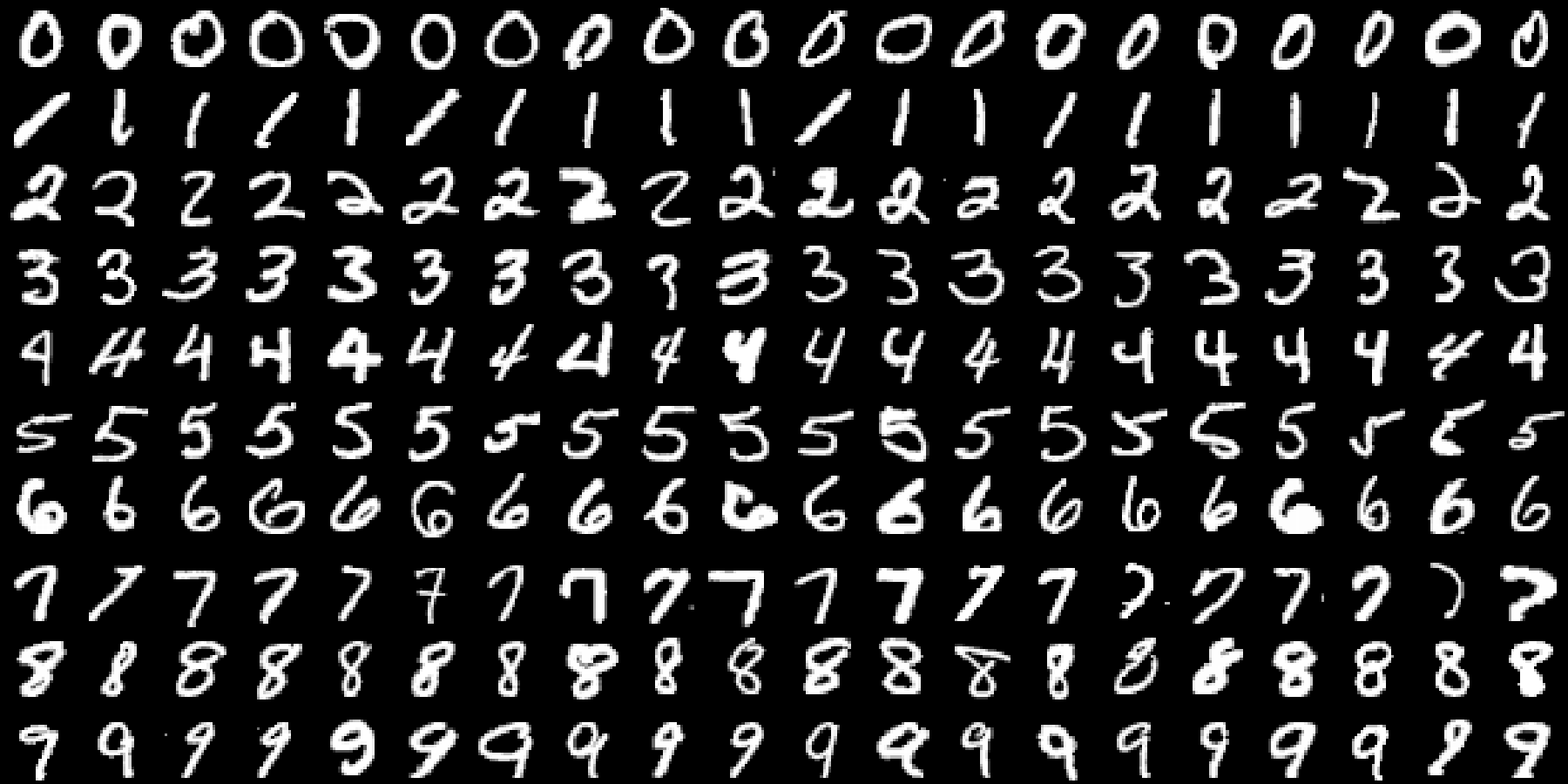
Figure 5.1: Example images in the MNIST database
There are 10 unique digits, so this is a multiclass classification problem.
- Remark.
-
The dataset is already “too easy” for testing of the state-of-the-art classifiers (see the notes below), but it’s a great educational example.
Accessing MNIST via the keras package
(which we will use throughout this chapter anyway) is easy:
library("keras")
mnist <- dataset_mnist()
X_train <- mnist$train$x
Y_train <- mnist$train$y
X_test  <- mnist$test$x
Y_test  <- mnist$test$y
X_train and X_test consist of 28×28 pixel images.
dim(X_train)## [1] 60000 28 28dim(X_test)## [1] 10000 28 28X_train and X_test are 3-dimensional arrays, think
of them as vectors of 60000 and 10000 matrices of size 28×28, respectively.
These are grey-scale images, with 0 = black, …, 255 = white:
range(X_train)## [1] 0 255Numerically, it’s more convenient to work with colour values converted to 0.0 = black, …, 1.0 = white:
X_train <- X_train/255
X_test  <- X_test/255
Y_train and Y_test are the corresponding integer labels:
length(Y_train)## [1] 60000length(Y_test)## [1] 10000table(Y_train) # label distribution in the training sample## Y_train
## 0 1 2 3 4 5 6 7 8 9
## 5923 6742 5958 6131 5842 5421 5918 6265 5851 5949table(Y_test) # label distribution in the test sample## Y_test
## 0 1 2 3 4 5 6 7 8 9
## 980 1135 1032 1010 982 892 958 1028 974 1009Here is how we can plot one of the digits (see Figure 5.2):
id <- 123 # image ID to show
image(z=t(X_train[id,,]), col=grey.colors(256, 0, 1),
    axes=FALSE, asp=1, ylim=c(1, 0))
legend("topleft", bg="white",
    legend=sprintf("True label=%d", Y_train[id]))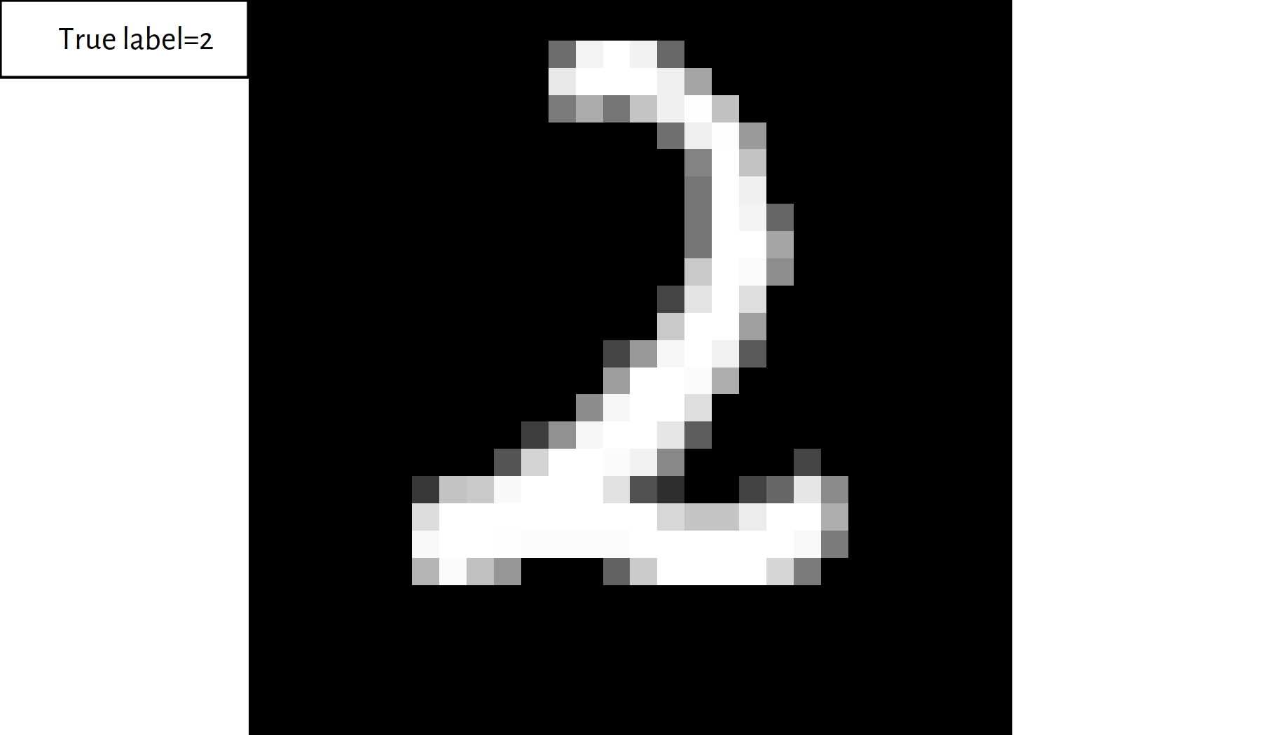
Figure 5.2: Example image from the MNIST dataset
5.2 Multinomial Logistic Regression
5.2.1 A Note on Data Representation
So… you may now be wondering “how do we construct an image classifier, this seems so complicated!”.
For a computer, (almost) everything is just numbers.
Instead of playing with \(n\) matrices, each of size 28×28, we may “flatten” the images so as to get \(n\) “long” vectors of length \(p=784\).
X_train2 <- matrix(X_train, ncol=28*28)
X_test2  <- matrix(X_test, ncol=28*28)
The classifiers studied here do not take the “spatial” positioning of the pixels into account anyway. Hence, now we’re back to our “comfort zone”.
- Remark.
-
(*) See, however, convolutional neural networks (CNNs), e.g., in (Goodfellow et al. 2016).
5.2.2 Extending Logistic Regression
Let us generalise the binary logistic regression model to a 10-class one (or, more generally, \(K\)-class one).
This time we will be modelling ten probabilities, with \(\Pr(Y=k|\mathbf{X},\mathbf{B})\) denoting the confidence that a given image \(\mathbf{X}\) is in fact the \(k\)-th digit:
\[ \begin{array}{lcl} \Pr(Y=0|\mathbf{X},\mathbf{B})&=&\dots\\ \Pr(Y=1|\mathbf{X},\mathbf{B})&=&\dots\\ &\vdots&\\ \Pr(Y=9|\mathbf{X},\mathbf{B})&=&\dots\\ \end{array} \]
where \(\mathbf{B}\) is the set of underlying model parameters (to be determined soon).
In binary logistic regression, the class probabilities are obtained by “cleverly normalising” (by means of the logistic sigmoid) the outputs of a linear model (so that we obtain a value in \([0,1]\)).
\[ \Pr(Y=1|\mathbf{X},\boldsymbol\beta)=\phi(\beta_0 + \beta_1 X_1 + \dots + \beta_p X_p)=\displaystyle\frac{1}{1+e^{-(\beta_0 + \beta_1 X_1 + \dots + \beta_p X_p)}} \]
In the multinomial case, we can use a separate linear model for each digit so that each \(\Pr(Y=k|\mathbf{X},\mathbf{B})\), \(k=0,1,\dots,9\), is given as a function of: \[\beta_{0,k} + \beta_{1,k} X_{1} + \dots + \beta_{p,k} X_{p}.\]
Therefore, instead of a parameter vector of length \((p+1)\), we will need a parameter matrix of size \((p+1)\times 10\) representing the model’s definition.
- Side note.
-
The upper case of \(\beta\) is \(B\).
Then, these 10 numbers will have to be normalised so as to they are all greater than \(0\) and sum to \(1\).
To maintain the spirit of the original model, we can apply \(e^{-(\beta_{0,k} + \beta_{1,k} X_{1} + \dots + \beta_{p,k} X_{p})}\) to get a positive value, because the co-domain of the exponential function \(t\mapsto e^t\) is \((0,\infty)\).
Then, dividing each output by the sum of all the outputs will guarantee that the total sum equals 1.
This leads to: \[ \begin{array}{lcl} \Pr(Y=0|\mathbf{X},\mathbf{B})&=&\displaystyle\frac{e^{-(\beta_{0,0} + \beta_{1,0} X_{1} + \dots + \beta_{p,0} X_{p})}}{\sum_{k=0}^9 e^{-(\beta_{0,k} + \beta_{1,k} X_{1} + \dots + \beta_{p,k} X_p)}},\\ \Pr(Y=1|\mathbf{X},\mathbf{B})&=&\displaystyle\frac{e^{-(\beta_{0,1} + \beta_{1,1} X_{1} + \dots + \beta_{p,1} X_{p})}}{\sum_{k=0}^9 e^{-(\beta_{0,k} + \beta_{1,k} X_{1} + \dots + \beta_{p,k} X_{p})}},\\ &\vdots&\\ \Pr(Y=9|\mathbf{X},\mathbf{B})&=&\displaystyle\frac{e^{-(\beta_{0,9} + \beta_{1,9} X_{1} + \dots + \beta_{p,9} X_{p})}}{\sum_{k=0}^9 e^{-(\beta_{0,k} + \beta_{1,k} X_{1} + \dots + \beta_{p,k} X_{p})}}.\\ \end{array} \]
This reduces to the binary logistic regression if we consider only the classes \(0\) and \(1\) and fix \(\beta_{0,0}=\beta_{1,0}=\dots=\beta_{p,0}=0\) (as \(e^0=1\)).
5.2.3 Softmax Function
The above transformation (that maps 10 arbitrary real numbers to positive ones that sum to 1) is called the softmax function (or softargmax).
softmax <- function(T) {
    T2 <- exp(T) # ignore the minus sign above
    T2/sum(T2)
}
round(rbind(
    softmax(c(0, 0, 10, 0, 0, 0, 0,  0, 0, 0)),
    softmax(c(0, 0, 10, 0, 0, 0, 10, 0, 0, 0)),
    softmax(c(0, 0, 10, 0, 0, 0, 9,  0, 0, 0)),
    softmax(c(0, 0, 10, 0, 0, 0, 9,  0, 0, 8))), 2)
## [,1] [,2] [,3] [,4] [,5] [,6] [,7] [,8] [,9] [,10]
## [1,] 0 0 1.00 0 0 0 0.00 0 0 0.00
## [2,] 0 0 0.50 0 0 0 0.50 0 0 0.00
## [3,] 0 0 0.73 0 0 0 0.27 0 0 0.00
## [4,] 0 0 0.67 0 0 0 0.24 0 0 0.095.2.4 One-Hot Encoding and Decoding
The ten class-belongingness-degrees can be decoded to obtain a single label by simply choosing the class that is assigned the highest probability.
y_pred <- softmax(c(0, 0, 10, 0, 0, 0, 9,  0, 0, 8))
round(y_pred, 2) # probabilities of Y=0, 1, 2, ..., 9
## [1] 0.00 0.00 0.67 0.00 0.00 0.00 0.24 0.00 0.00 0.09which.max(y_pred)-1 # 1..10 -> 0..9## [1] 2- Remark.
-
which.max(y)returns an indexksuch thaty[k]==max(y)(recall that in R the first element in a vector is at index1). Mathematically, we denote this operation as \(\mathrm{arg}\max_{k=1,\dots,K} y_k\).
To make processing the outputs of a logistic regression model more convenient, we will apply the so-called one-hot-encoding of the labels.
Here, each label will be represented as a 0-1 vector of 10 probabilities – with probability 1 corresponding to the true class only.
For instance:
y <- 2 # true class (this is just an example)
y2 <- rep(0, 10)
y2[y+1] <- 1 # +1 because we need 0..9 -> 1..10
y2  # one-hot-encoded y
## [1] 0 0 1 0 0 0 0 0 0 0To one-hot encode all the reference outputs in R, we start with a matrix of size \(n\times 10\) populated with “0”s:
Y_train2 <- matrix(0, nrow=length(Y_train), ncol=10)Next, for every \(i\), we insert a “1” in the \(i\)-th row
and the (Y_train[\(i\)]+1)-th column:
# Note the "+1" 0..9 -> 1..10
Y_train2[cbind(1:length(Y_train), Y_train+1)] <- 1- Remark.
-
In R, indexing a matrix
Awith a 2-column matrixB, i.e.,A[B], allows for an easy access toA[B[1,1], B[1,2]],A[B[2,1], B[2,2]],A[B[3,1], B[3,2]], …
Sanity check:
head(Y_train)## [1] 5 0 4 1 9 2head(Y_train2)## [,1] [,2] [,3] [,4] [,5] [,6] [,7] [,8] [,9] [,10]
## [1,] 0 0 0 0 0 1 0 0 0 0
## [2,] 1 0 0 0 0 0 0 0 0 0
## [3,] 0 0 0 0 1 0 0 0 0 0
## [4,] 0 1 0 0 0 0 0 0 0 0
## [5,] 0 0 0 0 0 0 0 0 0 1
## [6,] 0 0 1 0 0 0 0 0 0 0Let us generalise the above idea and write a function that can one-hot-encode any vector of integer labels:
one_hot_encode <- function(Y) {
    stopifnot(is.numeric(Y))
    c1 <- min(Y) # first class label
    cK <- max(Y) # last class label
    K <- cK-c1+1 # number of classes

    Y2 <- matrix(0, nrow=length(Y), ncol=K)
    Y2[cbind(1:length(Y), Y-c1+1)] <- 1
    Y2
}
Encode Y_train and Y_test:
Y_train2 <- one_hot_encode(Y_train)
Y_test2 <- one_hot_encode(Y_test)
5.2.5 Cross-entropy Revisited
Our classifier will be outputting \(K=10\) probabilities.
The true class labels are not one-hot-encoded so that they are represented as vectors of \(K-1\) zeros and a single one.
How to measure the “agreement” between these two?
In essence, we will be comparing the probability vectors as generated by a classifier, \(\hat{Y}\):
round(y_pred, 2)## [1] 0.00 0.00 0.67 0.00 0.00 0.00 0.24 0.00 0.00 0.09with the one-hot-encoded true probabilities, \(Y\):
y2## [1] 0 0 1 0 0 0 0 0 0 0It turns out that one of the definitions of cross-entropy introduced above already handles the case of multiclass classification: \[ E(\mathbf{B}) = -\frac{1}{n} \sum_{i=1}^n \log \Pr(Y=y_i|\mathbf{x}_{i,\cdot},\mathbf{B}). \] The smaller the probability corresponding to the ground-truth class outputted by the classifier, the higher the penalty, see Figure 5.3.
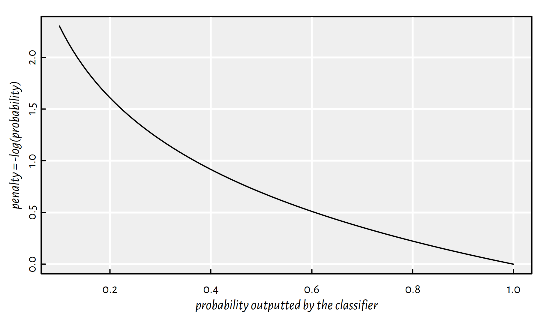
Figure 5.3: The less the classifier is confident about the prediction of the actually true label, the greater the penalty
To sum up, we will be solving the optimisation problem: \[ \min_{\mathbf{B}\in\mathbb{R}^{(p+1)\times 10}} -\frac{1}{n} \sum_{i=1}^n \log \Pr(Y=y_i|\mathbf{x}_{i,\cdot},\mathbf{B}). \] This has no analytical solution, but can be solved using iterative methods (see the chapter on optimisation).
(*) Side note: A single term in the above formula, \[ \log \Pr(Y=y_i|\mathbf{x}_{i,\cdot},\mathbf{B}) \] given:
y_pred– a vector of 10 probabilities generated by the model: \[ \left[\Pr(Y=0|\mathbf{x}_{i,\cdot},\mathbf{B})\ \Pr(Y=1|\mathbf{x}_{i,\cdot},\mathbf{B})\ \cdots\ \Pr(Y=9|\mathbf{x}_{i,\cdot},\mathbf{B})\right] \]y2– a one-hot-encoded version of the true label, \(y_i\), of the form: \[ \left[0\ 0\ \cdots\ 0\ 1\ 0\ \cdots\ 0\right] \]
can be computed as:
sum(y2*log(y_pred))## [1] -0.407825.2.6 Problem Formulation in Matrix Form (**)
The definition of a multinomial logistic regression model for a multiclass classification task involving classes \(\{1,2,\dots,K\}\) is slightly bloated.
Assuming that \(\mathbf{X}\in\mathbb{R}^{n\times p}\) is the input matrix, to compute the \(K\) predicted probabilities for the \(i\)-th input, \[ \left[ \hat{y}_{i,1}\ \hat{y}_{i,2}\ \cdots\ \hat{y}_{i,K} \right], \] given a parameter matrix \(\mathbf{B}^{(p+1)\times K}\), we apply: \[ \begin{array}{lcl} \hat{y}_{i,1}=\Pr(Y=1|\mathbf{x}_{i,\cdot},\mathbf{B})&=&\displaystyle\frac{e^{\beta_{0,1} + \beta_{1,1} x_{i,1} + \dots + \beta_{p,1} x_{i,p}}}{\sum_{k=1}^K e^{\beta_{0,k} + \beta_{1,k} x_{i,1} + \dots + \beta_{p,k} x_{i,p}}},\\ &\vdots&\\ \hat{y}_{i,K}=\Pr(Y=K|\mathbf{x}_{i,\cdot},\mathbf{B})&=&\displaystyle\frac{e^{\beta_{0,K} + \beta_{1,K} x_{i,1} + \dots + \beta_{p,K} x_{i,p}}}{\sum_{k=1}^K e^{\beta_{0,k} + \beta_{1,k} x_{i,1} + \dots + \beta_{p,k} x_{i,p}}}.\\ \end{array} \]
- Remark.
-
We have dropped the minus sign in the exponentiation for brevity of notation. Note that we can always map \(b_{j,k}'=-b_{j,k}\).
It turns out we can make use of matrix notation to tidy the above formulas.
Denote the linear combinations prior to computing the softmax function with: \[ \begin{array}{lcl} t_{i,1}&=&\beta_{0,1} + \beta_{1,1} x_{i,1} + \dots + \beta_{p,1} x_{i,p},\\ &\vdots&\\ t_{i,K}&=&\beta_{0,K} + \beta_{1,K} x_{i,1} + \dots + \beta_{p,K} x_{i,p}.\\ \end{array} \]
We have:
- \(x_{i,j}\) – the \(i\)-th observation, the \(j\)-th feature;
- \(\hat{y}_{i,k}\) – the \(i\)-th observation, the \(k\)-th class probability;
- \(\beta_{j,k}\) – the coefficient for the \(j\)-th feature when computing the \(k\)-th class.
Note that by augmenting \(\mathbf{\dot{X}}=[\boldsymbol{1}\ \mathbf{X}]\in\mathbb{R}^{n\times (p+1)}\) by adding a column of 1s, i.e., where \(\dot{x}_{i,0}=1\) and \(\dot{x}_{i,j}=x_{i,j}\) for all \(j\ge 1\) and all \(i\), we can write the above as: \[ \begin{array}{lclcl} t_{i,1}&=&\sum_{j=0}^p \dot{x}_{i,j}\, \beta_{j,1} &=& \dot{\mathbf{x}}_{i,\cdot}\, \boldsymbol\beta_{\cdot,1},\\ &\vdots&\\ t_{i,K}&=&\sum_{j=0}^p \dot{x}_{i,j}\, \beta_{j,K} &=& \dot{\mathbf{x}}_{i,\cdot}\, \boldsymbol\beta_{\cdot,K}.\\ \end{array} \]
We can get the \(K\) linear combinations all at once in the form of a row vector by writing: \[ \left[ t_{i,1}\ t_{i,2}\ \cdots\ t_{i,K} \right] = {\mathbf{x}_{i,\cdot}}\, \mathbf{B}. \]
Moreover, we can do that for all the \(n\) inputs by writing: \[ \mathbf{T}=\dot{\mathbf{X}}\,\mathbf{B}. \] Yes yes yes! This is a single matrix multiplication, we have \(\mathbf{T}\in\mathbb{R}^{n\times K}\).
To obtain \(\hat{\mathbf{Y}}\), we have to apply the softmax function on every row of \(\mathbf{T}\): \[ \hat{\mathbf{Y}}=\mathrm{softmax}\left( \dot{\mathbf{X}}\,\mathbf{B} \right). \]
That’s it. Take some time to appreciate the elegance of this notation.
Methods for minimising cross-entropy expressed in matrix form will be discussed in the next chapter.
5.3 Artificial Neural Networks
5.3.1 Artificial Neuron
A neuron can be thought of as a mathematical function, see Figure 5.4, which has its specific inputs and an output.
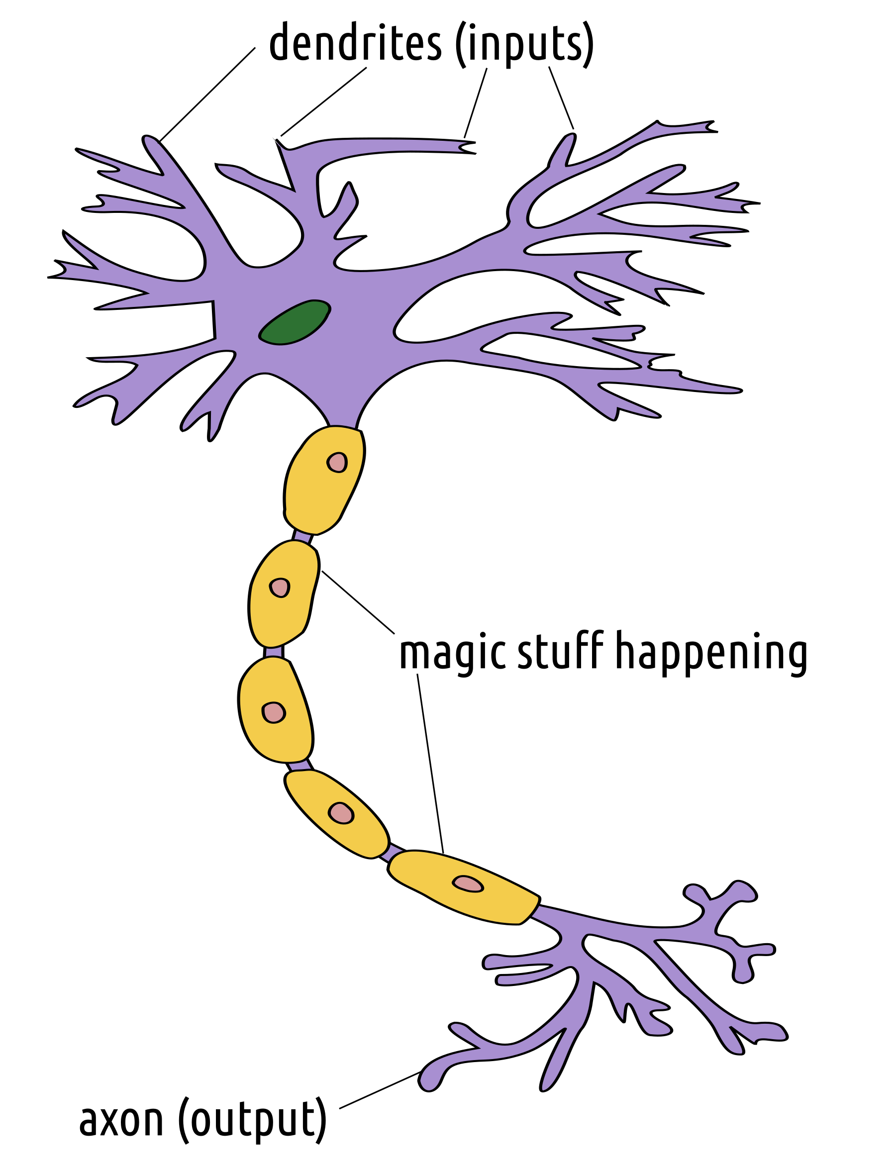
Figure 5.4: Neuron as a mathematical (black box) function; image based on: https://en.wikipedia.org/wiki/File:Neuron3.png by Egm4313.s12 at English Wikipedia, licensed under the Creative Commons Attribution-Share Alike 3.0 Unported license
The Linear Threshold Unit (McCulloch and Pitts, 1940s), the Perceptron (Rosenblatt, 1958) and the Adaptive Linear Neuron (Widrow and Hoff, 1960) were amongst the first models of an artificial neuron that could be used for the purpose of pattern recognition, see Figure 5.5. They can be thought of as processing units that compute a weighted sum of the inputs, which is then transformed by means of a nonlinear “activation” function.
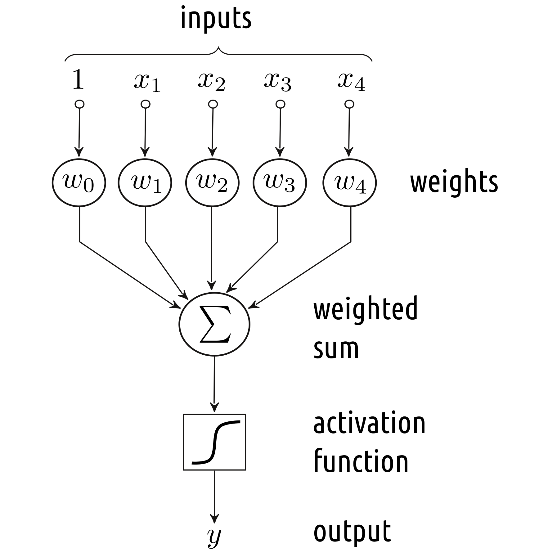
Figure 5.5: A simple model of an artificial neuron
5.3.2 Logistic Regression as a Neural Network
The above resembles our binary logistic regression model, where we determine a linear combination (a weighted sum) of \(p\) inputs and then transform it using the logistic sigmoid “activation” function. We can easily depict it in the Figure 5.4-style, see Figure 5.6.

Figure 5.6: Binary logistic regression
On the other hand, a multiclass logistic regression can be depicted as in Figure 5.7. In fact, we can consider it as an instance of a:
- single layer (there is only one processing step that consists of 10 units),
- densely connected (all the inputs are connected to all the components below),
- feed-forward (the outputs are generated by processing the inputs from “top” to “bottom”, there are no loops in the graph etc.)
artificial neural network that uses the softmax as the activation function.

Figure 5.7: Multinomial logistic regression
5.3.3 Example in R
To train such a neural network (i.e., fit a multinomial
logistic regression model),
we will use the keras package,
a wrapper around the (GPU-enabled) TensorFlow library.
The training of the model takes a few minutes (for more complex
models and bigger datasets – it could take hours/days).
Thus, it is wise to store the computed model (the \(\mathbf{B}\)
coefficient matrix and the accompanying keras’s auxiliary data)
for further reference:
file_name <- "datasets/mnist_keras_model1.h5"
if (!file.exists(file_name)) { # File doesn't exist -> compute
    set.seed(123)
    # Start with an empty model
    model1 <- keras_model_sequential()
    # Add a single layer with 10 units and softmax activation
    layer_dense(model1, units=10, activation="softmax")
    # We will be minimising the cross-entropy,
    # sgd == stochastic gradient descent, see the next chapter
    compile(model1, optimizer="sgd",
            loss="categorical_crossentropy")
    # Fit the model (slooooow!)
    fit(model1, X_train2, Y_train2, epochs=10)
    # Save the model for future reference
    save_model_hdf5(model1, file_name)
} else { # File exists -> reload the model
    model1 <- load_model_hdf5(file_name)
}
Let’s make predictions over the test set:
Y_pred2 <- predict(model1, X_test2)
round(head(Y_pred2), 2) # predicted class probabilities
## [,1] [,2] [,3] [,4] [,5] [,6] [,7] [,8] [,9] [,10]
## [1,] 0.00 0.00 0.00 0.00 0.00 0.00 0.00 1.00 0.00 0.00
## [2,] 0.01 0.00 0.93 0.01 0.00 0.01 0.04 0.00 0.00 0.00
## [3,] 0.00 0.96 0.02 0.00 0.00 0.00 0.00 0.00 0.01 0.00
## [4,] 1.00 0.00 0.00 0.00 0.00 0.00 0.00 0.00 0.00 0.00
## [5,] 0.00 0.00 0.01 0.00 0.91 0.00 0.01 0.01 0.01 0.05
## [6,] 0.00 0.98 0.00 0.00 0.00 0.00 0.00 0.00 0.01 0.00Then, we can one-hot-decode the output probabilities:
Y_pred <- apply(Y_pred2, 1, which.max)-1 # 1..10 -> 0..9
head(Y_pred, 20) # predicted outputs
## [1] 7 2 1 0 4 1 4 9 6 9 0 6 9 0 1 5 9 7 3 4head(Y_test, 20) # true outputs## [1] 7 2 1 0 4 1 4 9 5 9 0 6 9 0 1 5 9 7 3 4Accuracy on the test set:
mean(Y_test == Y_pred)## [1] 0.9169Performance metrics for each digit separately (see also Figure 5.8):
| i | Acc | Prec | Rec | F | TN | FN | FP | TP |
|---|---|---|---|---|---|---|---|---|
| 0 | 0.9924 | 0.94664 | 0.97755 | 0.96185 | 8966 | 22 | 54 | 958 |
| 1 | 0.9923 | 0.95920 | 0.97357 | 0.96633 | 8818 | 30 | 47 | 1105 |
| 2 | 0.9803 | 0.92214 | 0.88372 | 0.90252 | 8891 | 120 | 77 | 912 |
| 3 | 0.9802 | 0.89417 | 0.91188 | 0.90294 | 8881 | 89 | 109 | 921 |
| 4 | 0.9833 | 0.90148 | 0.93177 | 0.91637 | 8918 | 67 | 100 | 915 |
| 5 | 0.9793 | 0.91415 | 0.84753 | 0.87958 | 9037 | 136 | 71 | 756 |
| 6 | 0.9885 | 0.93142 | 0.94990 | 0.94057 | 8975 | 48 | 67 | 910 |
| 7 | 0.9834 | 0.92843 | 0.90856 | 0.91839 | 8900 | 94 | 72 | 934 |
| 8 | 0.9754 | 0.86473 | 0.88604 | 0.87525 | 8891 | 111 | 135 | 863 |
| 9 | 0.9787 | 0.90040 | 0.88702 | 0.89366 | 8892 | 114 | 99 | 895 |
Note how misleading the individual accuracies are! Averaging over the above table’s columns gives:
##     Acc    Prec     Rec       F
## 0.98338 0.91628 0.91575 0.91575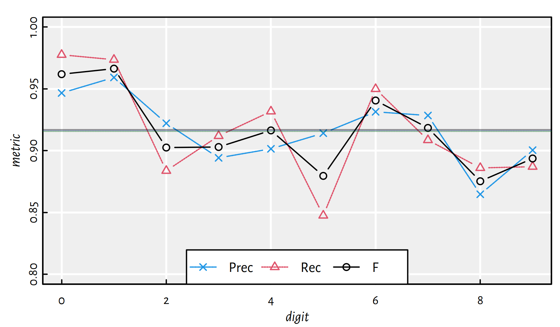
Figure 5.8: Performance metrics for multinomial logistic regression on MNIST
5.4 Deep Neural Networks
5.4.1 Introduction
In a brain, a neuron’s output is an input a bunch of other neurons. We could try aligning neurons into many interconnected layers. This leads to a structure like the one in Figure 5.9.
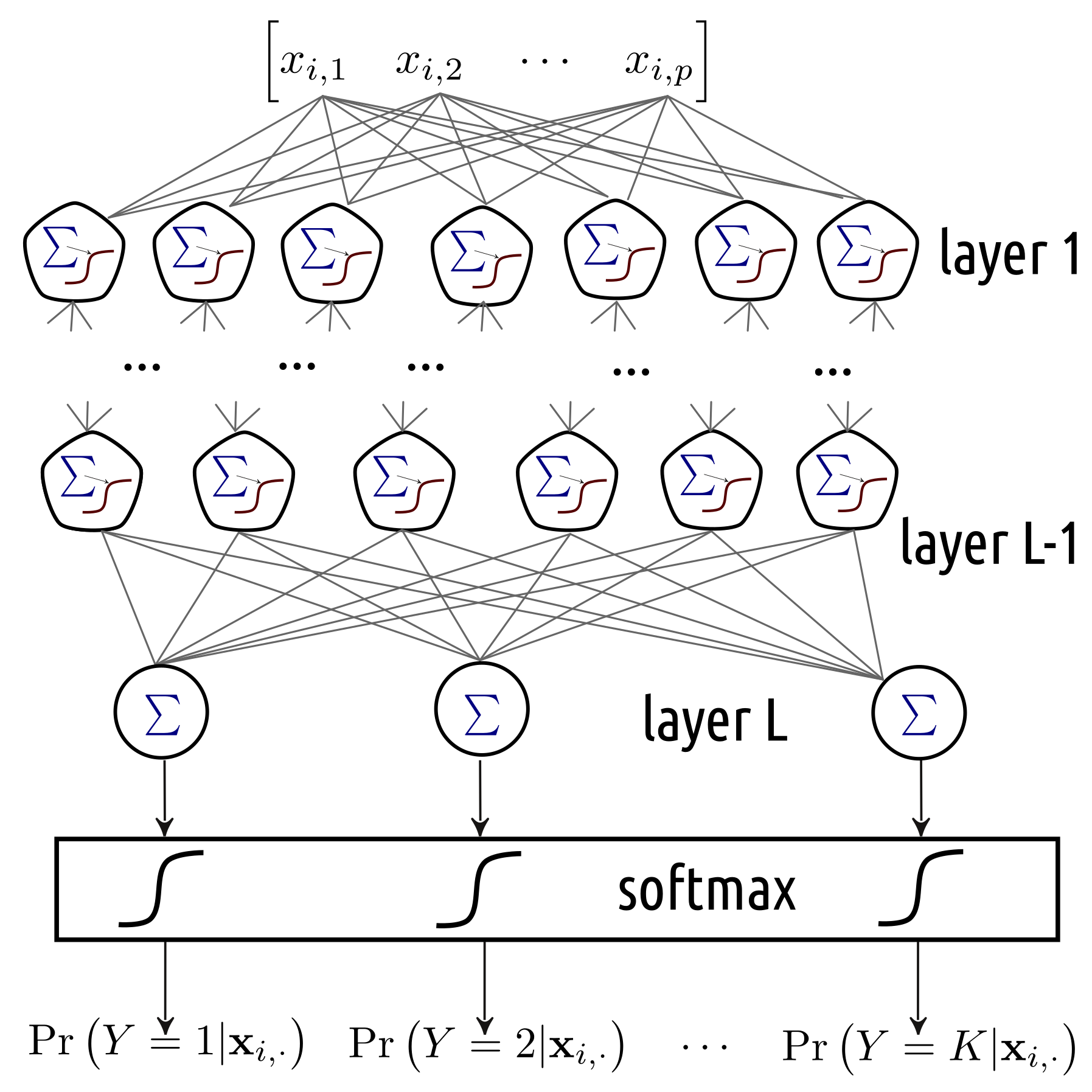
Figure 5.9: A multi-layer neural network
5.4.2 Activation Functions
Each layer’s outputs should be transformed by some non-linear activation function. Otherwise, we’d end up with linear combinations of linear combinations, which are linear combinations themselves.
Example activation functions that can be used in hidden (inner) layers:
relu– The rectified linear unit: \[\psi(t)=\max(t, 0),\]sigmoid– The logistic sigmoid: \[\phi(t)= \frac{1}{1 + \exp(-t)},\]tanh– The hyperbolic function: \[\mathrm{tanh}(t) = \frac{\exp(t) - \exp(-t)}{\exp(t) + \exp(-t)}.\]
There is not much difference between them, but some might be more convenient to handle numerically than the others, depending on the implementation.
5.4.3 Example in R - 2 Layers
Let’s construct a 2-layer Neural Network of the type 784-800-10:
file_name <- "datasets/mnist_keras_model2.h5"
if (!file.exists(file_name)) {
    set.seed(123)
    model2 <- keras_model_sequential()
    layer_dense(model2, units=800, activation="relu")
    layer_dense(model2, units=10,  activation="softmax")
    compile(model2, optimizer="sgd",
            loss="categorical_crossentropy")
    fit(model2, X_train2, Y_train2, epochs=10)
    save_model_hdf5(model2, file_name)
} else {
    model2 <- load_model_hdf5(file_name)
}

Y_pred2 <- predict(model2, X_test2)
Y_pred <- apply(Y_pred2, 1, which.max)-1 # 1..10 -> 0..9
mean(Y_test == Y_pred) # accuracy on the test set
## [1] 0.9583Performance metrics for each digit separately, see also Figure 5.10:
| i | Acc | Prec | Rec | F | TN | FN | FP | TP |
|---|---|---|---|---|---|---|---|---|
| 0 | 0.9948 | 0.96215 | 0.98571 | 0.97379 | 8982 | 14 | 38 | 966 |
| 1 | 0.9962 | 0.98156 | 0.98502 | 0.98329 | 8844 | 17 | 21 | 1118 |
| 2 | 0.9911 | 0.96000 | 0.95349 | 0.95673 | 8927 | 48 | 41 | 984 |
| 3 | 0.9898 | 0.94773 | 0.95149 | 0.94960 | 8937 | 49 | 53 | 961 |
| 4 | 0.9919 | 0.95829 | 0.95927 | 0.95878 | 8977 | 40 | 41 | 942 |
| 5 | 0.9911 | 0.95470 | 0.94507 | 0.94986 | 9068 | 49 | 40 | 843 |
| 6 | 0.9920 | 0.94888 | 0.96868 | 0.95868 | 8992 | 30 | 50 | 928 |
| 7 | 0.9906 | 0.95517 | 0.95331 | 0.95424 | 8926 | 48 | 46 | 980 |
| 8 | 0.9899 | 0.95421 | 0.94148 | 0.94780 | 8982 | 57 | 44 | 917 |
| 9 | 0.9892 | 0.95643 | 0.93558 | 0.94589 | 8948 | 65 | 43 | 944 |
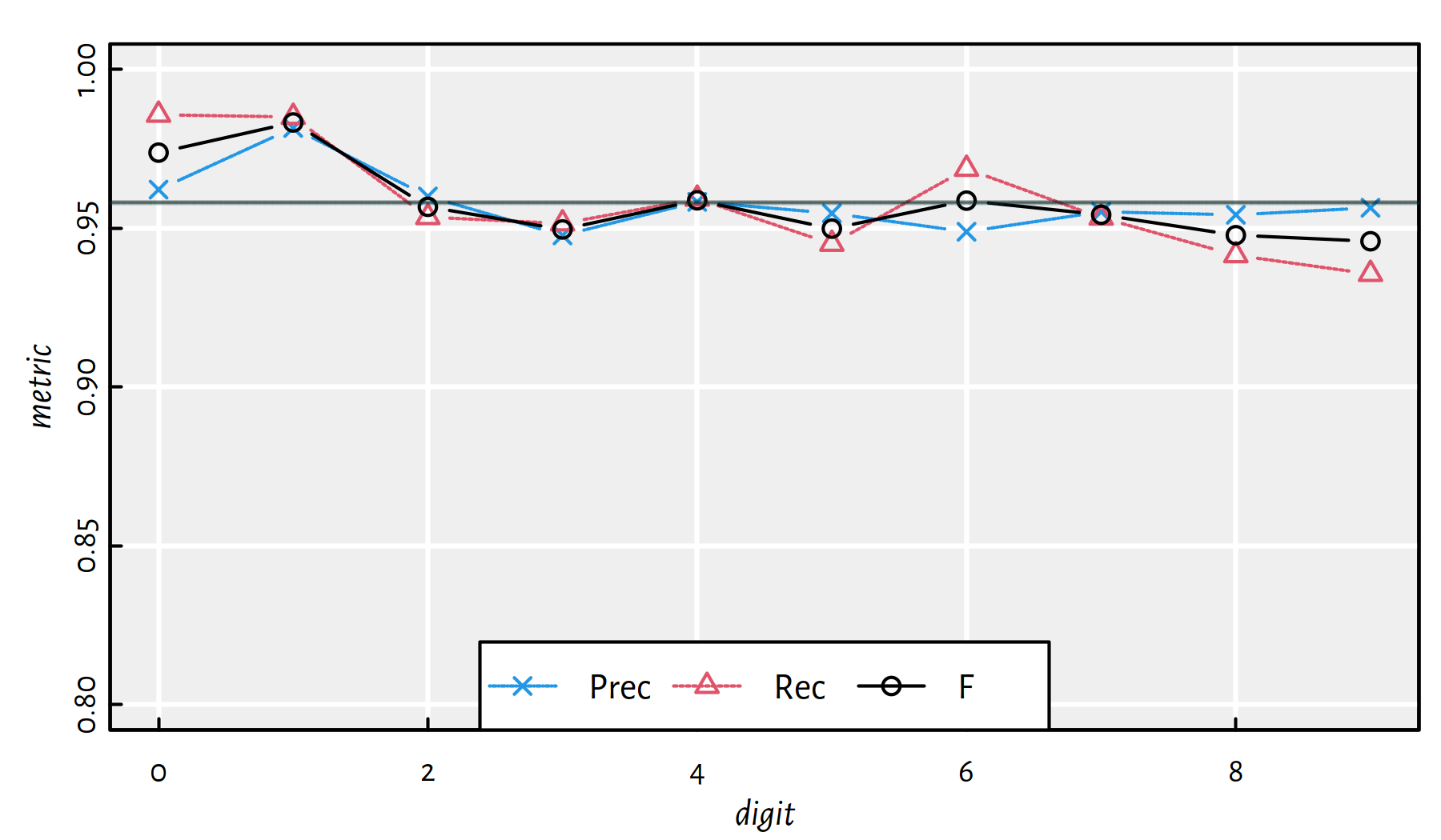
Figure 5.10: Performance metrics for a 2-layer net 784-800-10 [relu] on MNIST
5.4.4 Example in R - 6 Layers
How about a 6-layer Deep Neural Network like 784-2500-2000-1500-1000-500-10? Here you are:
file_name <- "datasets/mnist_keras_model3.h5"
if (!file.exists(file_name)) {
    set.seed(123)
    model3 <- keras_model_sequential()
    layer_dense(model3, units=2500, activation="relu")
    layer_dense(model3, units=2000, activation="relu")
    layer_dense(model3, units=1500, activation="relu")
    layer_dense(model3, units=1000, activation="relu")
    layer_dense(model3, units=500,  activation="relu")
    layer_dense(model3, units=10,   activation="softmax")
    compile(model3, optimizer="sgd",
            loss="categorical_crossentropy")
    fit(model3, X_train2, Y_train2, epochs=10)
    save_model_hdf5(model3, file_name)
} else {
    model3 <- load_model_hdf5(file_name)
}

Y_pred2 <- predict(model3, X_test2)
Y_pred <- apply(Y_pred2, 1, which.max)-1 # 1..10 -> 0..9
mean(Y_test == Y_pred) # accuracy on the test set
## [1] 0.9769Performance metrics for each digit separately, see also Figure 5.11.
| i | Acc | Prec | Rec | F | TN | FN | FP | TP |
|---|---|---|---|---|---|---|---|---|
| 0 | 0.9964 | 0.97295 | 0.99082 | 0.98180 | 8993 | 9 | 27 | 971 |
| 1 | 0.9980 | 0.99206 | 0.99031 | 0.99118 | 8856 | 11 | 9 | 1124 |
| 2 | 0.9948 | 0.99000 | 0.95930 | 0.97441 | 8958 | 42 | 10 | 990 |
| 3 | 0.9948 | 0.97239 | 0.97624 | 0.97431 | 8962 | 24 | 28 | 986 |
| 4 | 0.9951 | 0.97846 | 0.97149 | 0.97496 | 8997 | 28 | 21 | 954 |
| 5 | 0.9963 | 0.97553 | 0.98318 | 0.97934 | 9086 | 15 | 22 | 877 |
| 6 | 0.9965 | 0.98224 | 0.98121 | 0.98172 | 9025 | 18 | 17 | 940 |
| 7 | 0.9941 | 0.95837 | 0.98541 | 0.97170 | 8928 | 15 | 44 | 1013 |
| 8 | 0.9939 | 0.96534 | 0.97228 | 0.96880 | 8992 | 27 | 34 | 947 |
| 9 | 0.9939 | 0.98073 | 0.95837 | 0.96942 | 8972 | 42 | 19 | 967 |
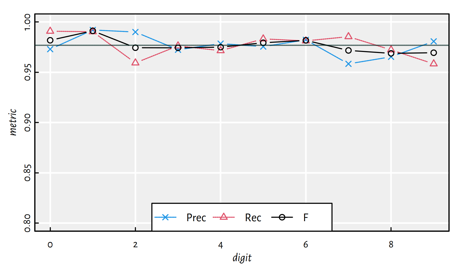
Figure 5.11: Performance metrics for a 6-layer net 784-2500-2000-1500-1000-500-10 [relu] on MNIST
Test the performance of different neural network
architectures (different number of layers, different number
of neurons in each layer etc.). Yes, it’s more art than science!
Many tried to come up with various “rules of thumb”,
see, for example, the comp.ai.neural-nets FAQ (Sarle et al. 2002) at
http://www.faqs.org/faqs/ai-faq/neural-nets/part3/preamble.html,
but what works well in one problem might not be generalisable
to another one.
5.5 Preprocessing of Data
5.5.1 Introduction
Do not underestimate the power of appropriate data preprocessing — deep neural networks are not a universal replacement for a data engineer’s hard work!
On top of that, they are not interpretable – these are merely black-boxes.
Among the typical transformations of the input images we can find:
- normalisation of colours (setting brightness, stretching contrast, etc.),
- repositioning of the image (centring),
- deskewing (see below),
- denoising (e.g., by blurring).
Another frequently applied technique concerns an expansion of the training data — we can add “artificially contaminated” images to the training set (e.g., slightly rotated digits) so as to be more ready to whatever will be provided in the test test.
5.5.2 Image Deskewing
Deskewing of images (“straightening” of the digits) is amongst the most typical transformations that can be applied on MNIST.
Unfortunately, we don’t have (yet) the necessary mathematical background to discuss this operation in very detail.
Luckily, we can apply it on each image anyway.
See the GitHub repository at https://github.com/gagolews/Playground.R
for an example notebook and the deskew.R script.
# See https://github.com/gagolews/Playground.R
source("~/R/Playground.R/deskew.R")
# new_image <- deskew(old_image)
Figure 5.12: Deskewing of the MNIST digits
Let’s take a look at Figure 5.12. In each pair, the left image (black background) is the original one, and the right image (palette inverted for purely dramatic effects) is its deskewed version.
Below we deskew each image in the training as well as in the test sample. This also takes a long time, so let’s store the resulting objects for further reference:
file_name <- "datasets/mnist_deskewed_train.rds"
if (!file.exists(file_name)) {
    Z_train <- X_train
    for (i in 1:dim(Z_train)[1]) {
        Z_train[i,,] <- deskew(Z_train[i,,])
    }
    Z_train2 <- matrix(Z_train, ncol=28*28)
    saveRDS(Z_train2, file_name)
} else {
    Z_train2 <- readRDS(file_name)
}

file_name <- "datasets/mnist_deskewed_test.rds"
if (!file.exists(file_name)) {
    Z_test <- X_test
    for (i in 1:dim(Z_test)[1]) {
        Z_test[i,,] <- deskew(Z_test[i,,])
    }
    Z_test2 <- matrix(Z_test, ncol=28*28)
    saveRDS(Z_test2, file_name)
} else {
    Z_test2 <- readRDS(file_name)
}- Remark.
-
RDS in a compressed file format used by R for object serialisation (quickly storing its verbatim copies so that they can be reloaded at any time).
Multinomial logistic regression model (1-layer NN):
file_name <- "datasets/mnist_keras_model1d.h5"
if (!file.exists(file_name)) {
    set.seed(123)
    model1d <- keras_model_sequential()
    layer_dense(model1d, units=10, activation="softmax")
    compile(model1d, optimizer="sgd",
            loss="categorical_crossentropy")
    fit(model1d, Z_train2, Y_train2, epochs=10)
    save_model_hdf5(model1d, file_name)
} else {
    model1d <- load_model_hdf5(file_name)
}

Y_pred2 <- predict(model1d, Z_test2)
Y_pred <- apply(Y_pred2, 1, which.max)-1 # 1..10 -> 0..9
mean(Y_test == Y_pred) # accuracy on the test set
## [1] 0.9488Performance metrics for each digit separately, see also Figure 5.13.
| i | Acc | Prec | Rec | F | TN | FN | FP | TP |
|---|---|---|---|---|---|---|---|---|
| 0 | 0.9939 | 0.95450 | 0.98469 | 0.96936 | 8974 | 15 | 46 | 965 |
| 1 | 0.9959 | 0.98236 | 0.98150 | 0.98193 | 8845 | 21 | 20 | 1114 |
| 2 | 0.9878 | 0.95409 | 0.92636 | 0.94002 | 8922 | 76 | 46 | 956 |
| 3 | 0.9904 | 0.95069 | 0.95446 | 0.95257 | 8940 | 46 | 50 | 964 |
| 4 | 0.9888 | 0.94118 | 0.94501 | 0.94309 | 8960 | 54 | 58 | 928 |
| 5 | 0.9905 | 0.94426 | 0.94955 | 0.94690 | 9058 | 45 | 50 | 847 |
| 6 | 0.9905 | 0.95565 | 0.94468 | 0.95013 | 9000 | 53 | 42 | 905 |
| 7 | 0.9892 | 0.96000 | 0.93385 | 0.94675 | 8932 | 68 | 40 | 960 |
| 8 | 0.9855 | 0.91162 | 0.94251 | 0.92680 | 8937 | 56 | 89 | 918 |
| 9 | 0.9851 | 0.92914 | 0.92270 | 0.92591 | 8920 | 78 | 71 | 931 |
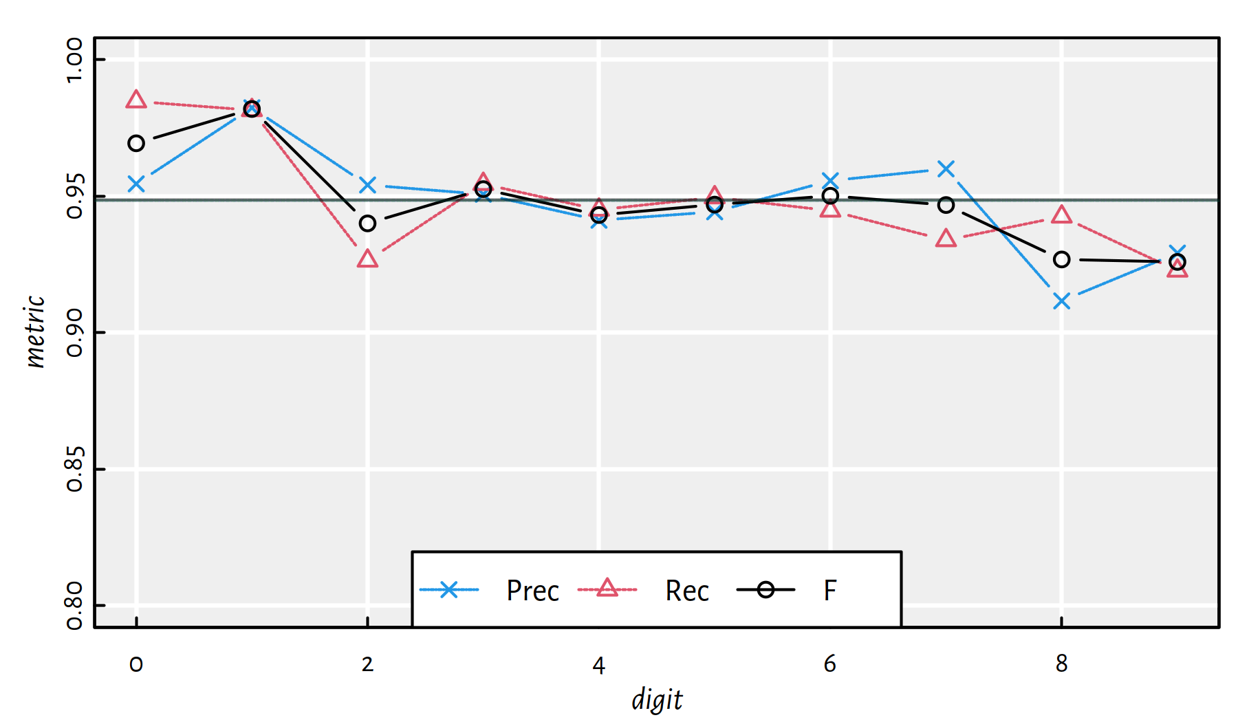
Figure 5.13: Performance of Multinomial Logistic Regression on the deskewed MNIST
5.5.3 Summary of All the Models Considered
Let’s summarise the quality of all the considered classifiers. Figure 5.14 gives the F-measures, for each digit separately.
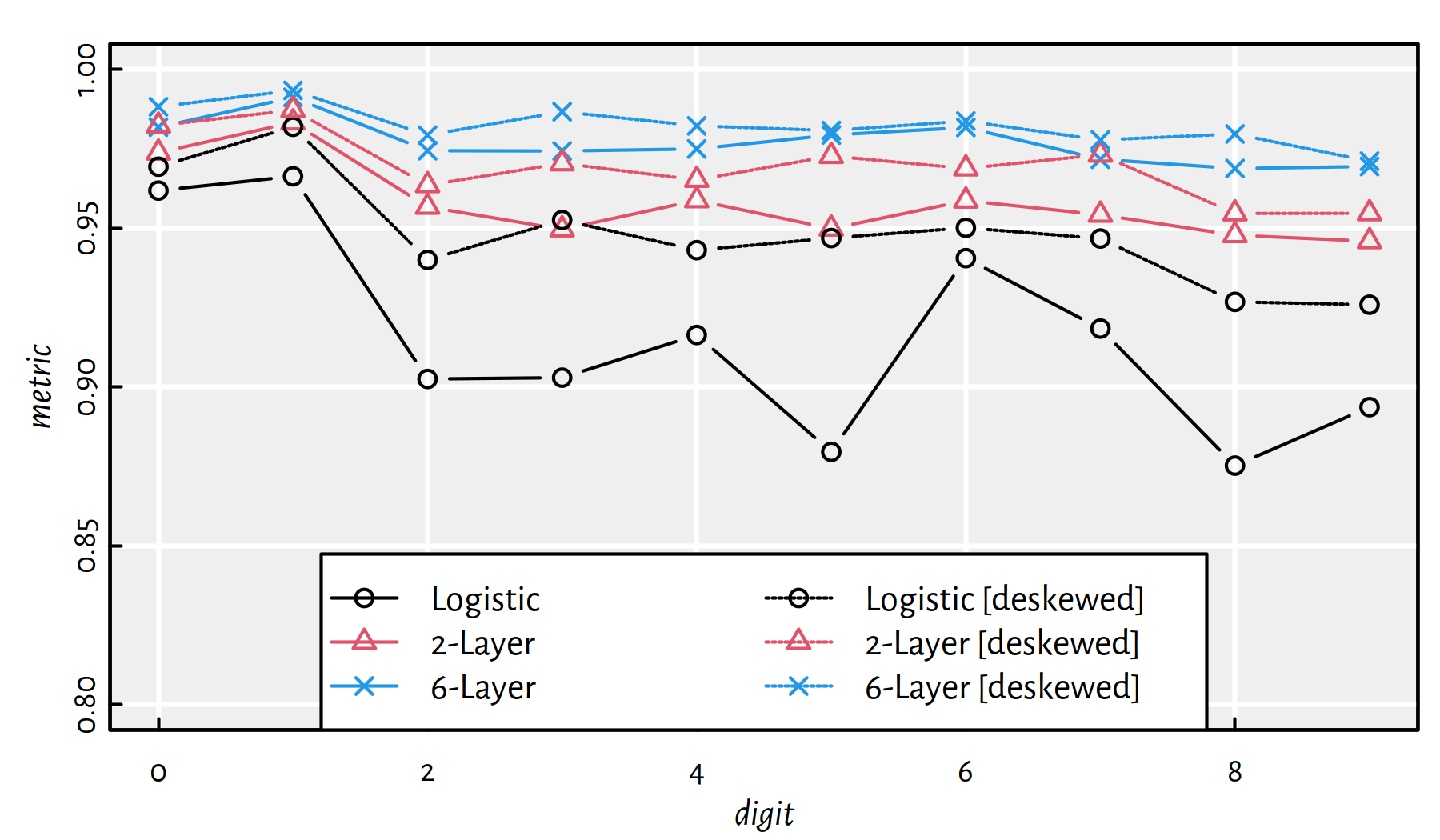
Figure 5.14: Summary of F-measures for each classified digit and every method
Note that the applied preprocessing of data increased the prediction accuracy.
The same information can also be included on a heat map
which is depicted in Figure 5.15
(see the image() function in R).
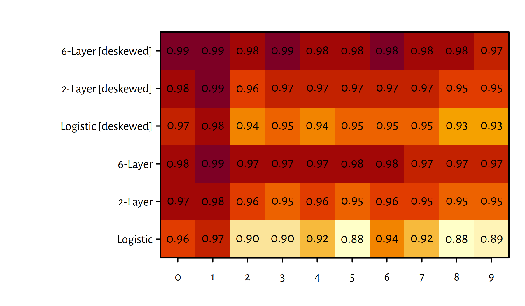
Figure 5.15: A heat map of F-measures for each classified digit and each method
5.6 Outro
5.6.1 Remarks
We have discussed a multinomial logistic regression model as a generalisation of the binary one.
This in turn is a special case of feed-forward neural networks.
There’s a lot of hype (again…) for deep neural networks in many applications, including vision, self-driving cars, natural language processing, speech recognition etc.
Many different architectures of neural networks and types of units are being considered in theory and in practice, e.g.:
- convolutional neural networks apply a series of signal (e.g., image) transformations in first layers, they might actually “discover” deskewing automatically etc.;
- recurrent neural networks can imitate long/short-term memory that can be used for speech synthesis and time series prediction.
Main drawbacks of deep neural networks:
- learning is very slow, especially with very deep architectures (days, weeks);
- models are not explainable (black boxes) and hard to debug;
- finding good architectures is more art than science (maybe: more of a craftsmanship even);
- sometimes using deep neural network is just an excuse for being too lazy to do proper data cleansing and pre-processing.
There are many issues and challenges that are tackled in more advanced AI/ML courses and books, such as (Goodfellow et al. 2016).
5.6.2 Beyond MNIST
The MNIST dataset is a classic, although its use in deep learning research is nowadays discouraged – the dataset is not considered challenging anymore – state of the art classifiers can reach \(99.8\%\) accuracy.
See Zalando’s Fashion-MNIST (by Kashif Rasul & Han Xiao) at https://github.com/zalandoresearch/fashion-mnist for a modern replacement.
Alternatively, take a look at CIFAR-10 and CIFAR-100 (https://www.cs.toronto.edu/~kriz/cifar.html) by A. Krizhevsky et al. or at ImageNet (http://image-net.org/index) for an even greater challenge.
5.6.3 Further Reading
Recommended further reading: (James et al. 2017: Chapter 11), (Sarle et al. 2002) and (Goodfellow et al. 2016)
See also the keras package tutorials available at:
https://cran.r-project.org/web/packages/keras/index.html
and https://keras.rstudio.com.