6 Continuous Optimisation with Iterative Algorithms (*)
These lecture notes are distributed in the hope that they will be useful. Any bug reports are appreciated.
6.1 Introduction
6.1.1 Optimisation Problems
Mathematical optimisation (a.k.a. mathematical programming) deals with the study of algorithms to solve problems related to selecting the best element amongst the set of available alternatives.
Most frequently “best” is expressed in terms of an error or goodness of fit measure: \[ f:\mathbb{D}\to\mathbb{R} \] called an objective function, where \(\mathbb{D}\) is the search space (problem domain, feasible set).
An optimisation task deals with finding an element \(\mathbf{x}\in \mathbb{D}\) amongst the set of possible candidate solutions, that minimises or maximises \(f\):
\[ \min_{\mathbf{x}\in \mathbb{D}} f(\mathbf{x}) \quad\text{or}\quad\max_{\mathbf{x}\in \mathbb{D}} f(\mathbf{x}), \]
In this chapter we will deal with unconstrained continuous optimisation, i.e., we will assume the search space is \(\mathbb{D}=\mathbb{R}^p\) for some \(p\) – we’ll be optimising over \(p\) real-valued parameters.
6.1.2 Example Optimisation Problems in Machine Learning
In multiple linear regression we were minimising the sum of squared residuals \[ \min_{\boldsymbol\beta\in\mathbb{R}^p} \sum_{i=1}^n \left( \beta_0 + \beta_1 x_{i,1}+\dots+\beta_p x_{i,p} - y_i \right)^2. \]
In binary logistic regression we were minimising the cross-entropy: \[ \min_{\boldsymbol\beta\in\mathbb{R}^p} -\frac{1}{n} \sum_{i=1}^n \left(\begin{array}{r} y_i \log \left(\frac{1}{1+e^{-(\beta_0 + \beta_1 x_{i,1}+\dots+\beta_p x_{i,p}}} \right)\\ + (1-y_i)\log \left(\frac{e^{-(\beta_0 + \beta_1 x_{i,1}+\dots+\beta_p x_{i,p}}}{1+e^{-(\beta_0 + \beta_1 x_{i,1}+\dots+\beta_p x_{i,p})}}\right) \end{array}\right). \]
6.1.3 Types of Minima and Maxima
Note that minimising \(f\) is the same as maximising \(\bar{f}=-f\).
In other words, \(\min_{\mathbf{x}\in \mathbb{D}} f(\mathbf{x})\) and \(\max_{\mathbf{x}\in \mathbb{D}} -f(\mathbf{x})\) represent the same optimisation problems (and hence have identical solutions).
- Definition.
-
A minimum of \(f\) is a point \(\mathbf{x}^*\) such that \(f(\mathbf{x}^*)\le f(\mathbf{x})\) for all \(\mathbf{x}\in \mathbb{D}\). On the other hand, a maximum of \(f\) is a point \(\mathbf{x}^*\) such that \(f(\mathbf{x}^*)\ge f(\mathbf{x})\) for all \(\mathbf{x}\in \mathbb{D}\).
Assuming that \(\mathbb{D}=\mathbb{R}\), Figure 6.1 shows an example objective function, \(f:\mathbb{D}\to\mathbb{R}\), that has a minimum at \({x}^*=1\) with \(f(x^*)=-2\).
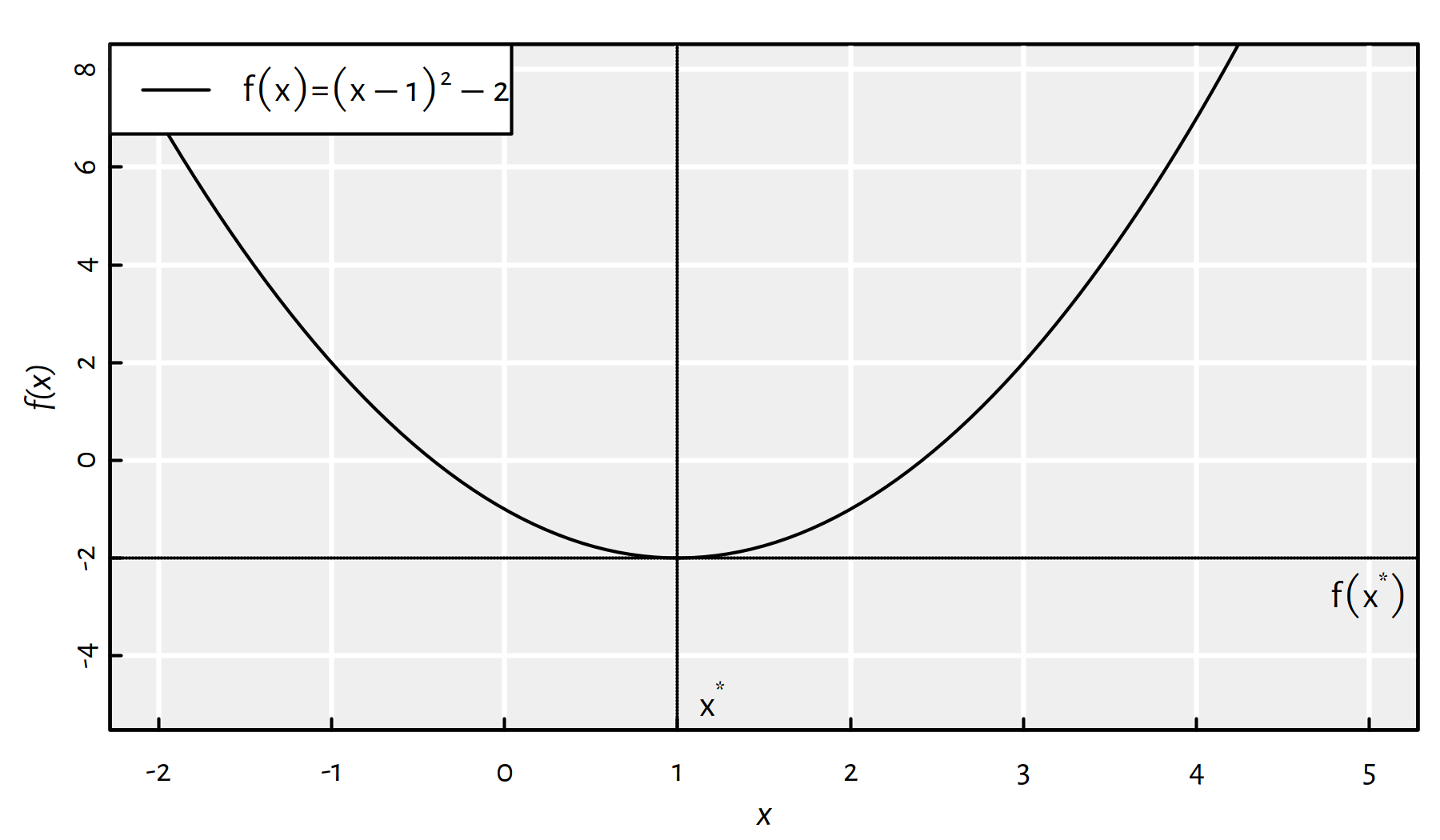
Figure 6.1: A function with the global minimum at \({x}^*=1\)
- Remark.
-
We can denote these two facts as follows:
- \((\min_{x\in \mathbb{R}} f(x))=-2\) (value of \(f\) at the minimum is \(-2\)),
- \((\mathrm{arg}\min_{x\in \mathbb{R}} f(x))=1\) (location of the minimum, i.e., argument minimum, is \(1\)).
By definition, a minimum/maximum might not necessarily be unique. This depends on a problem.
Assuming that \(\mathbb{D}=\mathbb{R}\), Figure 6.2 gives an example objective function, \(f:\mathbb{D}\to\mathbb{R}\), that has multiple minima; every \({x}^*\in[1-\sqrt{2},1+\sqrt{2}]\) yields \(f(x^*)=0\).
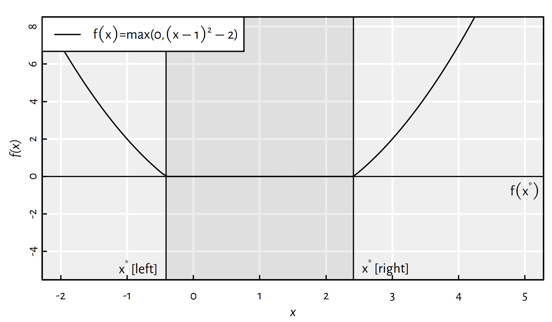
Figure 6.2: A function that has multiple minima
- Remark.
-
If this was the case of some machine learning problem, it would mean that we could have many equally well-performing models, and hence many equivalent explanations of the same phenomenon.
Moreover, it may happen that a function has multiple local minima, compare Figure 6.3.
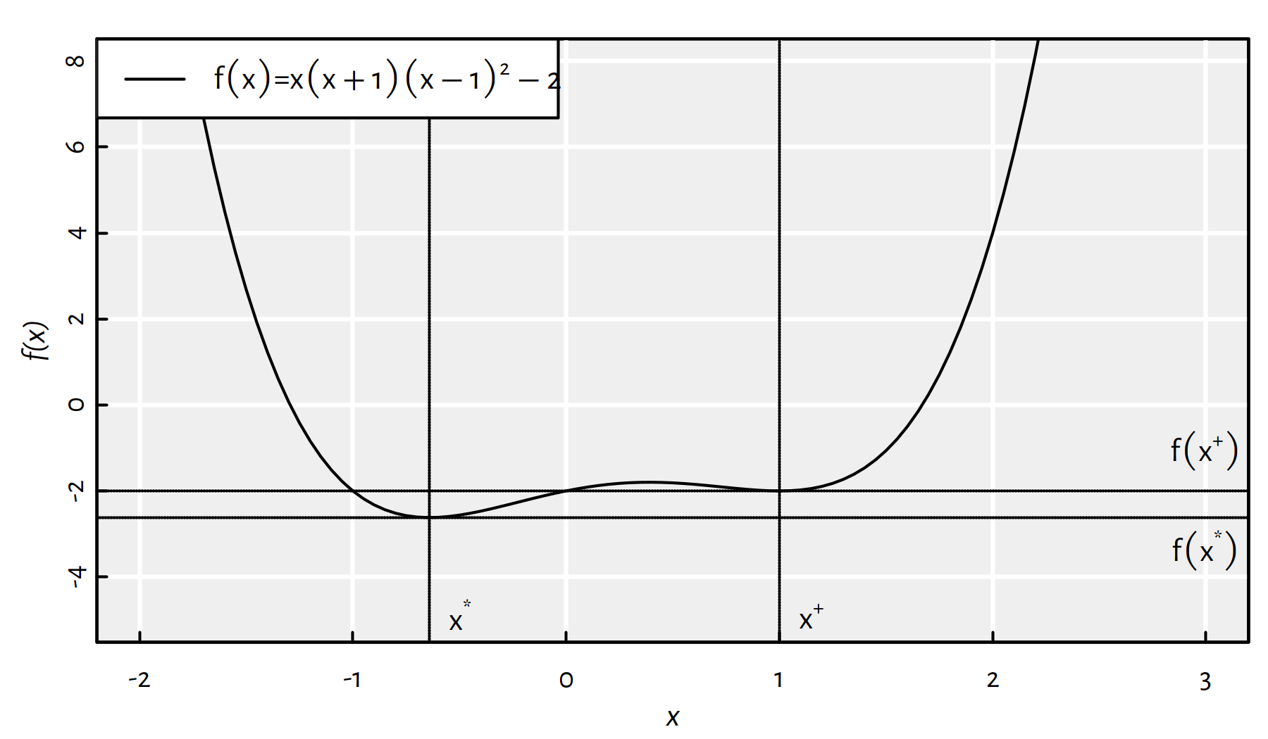
Figure 6.3: A function with two local minima
- Definition.
-
We say that \(f\) has a local minimum at \(\mathbf{x}^+\in \mathbb{D}\), if for some neighbourhood \(B(\mathbf{x}^+)\) of \(\mathbf{x}^+\) it holds \(f(\mathbf{x}^+) \le f(\mathbf{x})\) for each \(\mathbf{x}\in B(\mathbf{x}^+)\).
-
If \(\mathbb{D}=\mathbb{R}\), by neighbourhood \(B(x)\) of \(x\) we mean an open interval centred at \(x\) of width \(2r\) for some small \(r>0\), i.e., \((x-r, x+r)\)
- Definition.
-
(*) If \(\mathbb{D}=\mathbb{R}^p\) (for any \(p\ge 1\)), by neighbourhood \(B(\mathbf{x})\) of \(\mathbf{x}\) we mean an open ball centred at \(\mathbf{x}^+\) of some small radius \(r>0\), i.e., \(\{\mathbf{y}: \|\mathbf{x}-\mathbf{y}\|<r\}\) (read: the set of all the points with Euclidean distances to \(\mathbf{x}\) less than \(r\)).
To avoid ambiguity, the “true” minimum (a point \(\mathbf{x}^*\) such that \(f(\mathbf{x}^*)\le f({x})\) for all \(\mathbf{x}\in \mathbb{D}\)) is sometimes also referred to as a global minimum.
- Remark.
-
Of course, the global minimum is also a function’s local minimum.
The existence of local minima is problematic as most of the optimisation methods might get stuck there and fail to return the global one.
Moreover, we cannot often be sure if the result returned by an algorithm is indeed a global minimum. Maybe there exists a better solution that hasn’t been considered yet? Or maybe the function is very noisy (see Figure 6.4)?
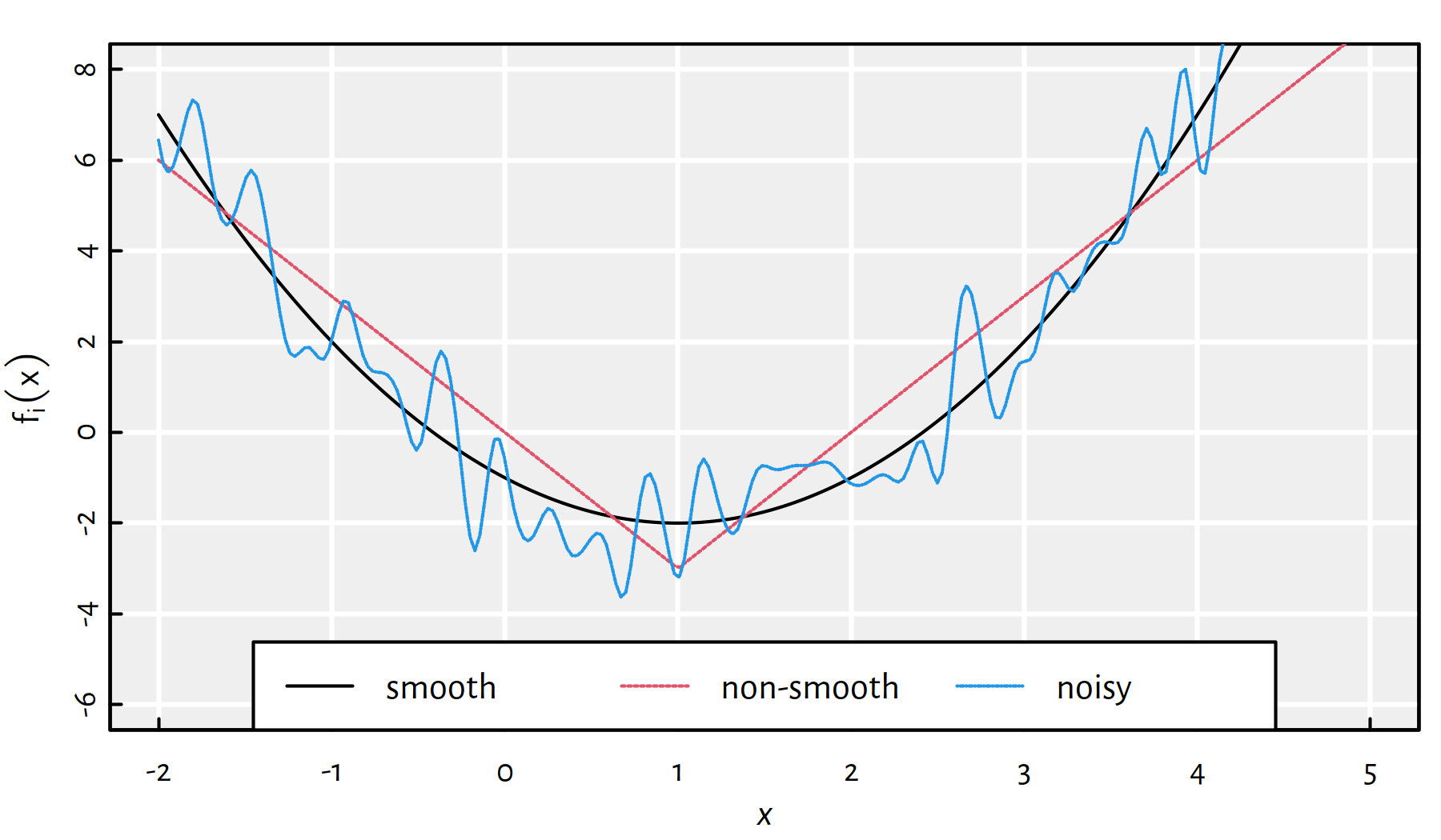
Figure 6.4: Smooth vs. non-smooth vs. noisy objective functions
6.1.4 Example Objective over a 2D Domain
Of course, our objective function does not necessarily have to be defined over a one-dimensional domain.
For example, consider the following function: \[ g(x_1,x_2)=\log\left((x_1^{2}+x_2-5)^{2}+(x_1+x_2^{2}-3)^{2}+x_1^2-1.60644\dots\right) \]
g  <- function(x1, x2)
    log((x1^2+x2-5)^2+(x1+x2^2-3)^2+x1^2-1.60644366086443841)
x1 <- seq(-5, 5, length.out=100)
x2 <- seq(-5, 5, length.out=100)
# outer() expands two vectors to form a 2D grid
# and applies a given function on each point
y  <- outer(x1, x2, g)
There are four local minima:
| x1 | x2 | f(x1,x2) |
|---|---|---|
| 2.2780 | -0.61343 | 1.3564 |
| -2.6123 | -2.34546 | 1.7051 |
| 1.7988 | 1.19879 | 0.6955 |
| -1.5423 | 2.15641 | 0.0000 |
The global minimum is at \(\mathbf{x}^*=(x_1^*, x_2^*)\) as below:
g(-1.542255693195422641930153, 2.156405289793087261832605)## [1] 0Let’s explore various ways of depicting \(f\) first. A contour plot and a heat map are given in Figure 6.5.
par(mfrow=c(1,2)) # 2 in 1
# lefthand plot:
contour(x1, x2, y, nlevels=25)
points(-1.54226, 2.15641, col=2, pch=3)
# righthand plot:
image(x1, x2, y)
contour(x1, x2, y, add=TRUE)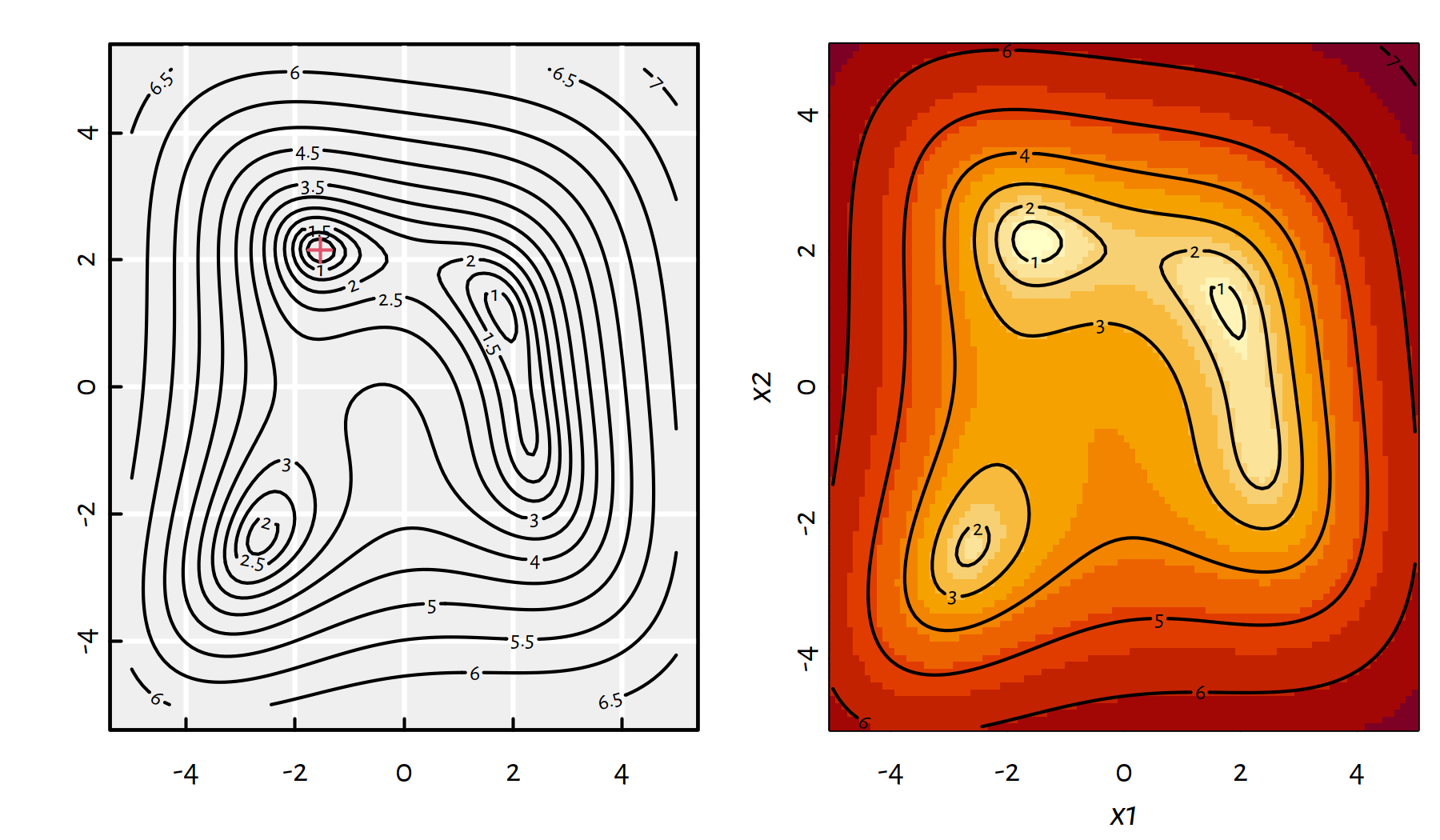
Figure 6.5: A contour plot and a heat map of \(g(x_1,x_2)\)
Two perspective plots (views from different angles) are given in Figure 6.6.
par(mfrow=c(1,2)) # 2 in 1
persp(x1, x2, y, phi=30, theta=-5, shade=2, border=NA)
persp(x1, x2, y, phi=30, theta=75, shade=2, border=NA)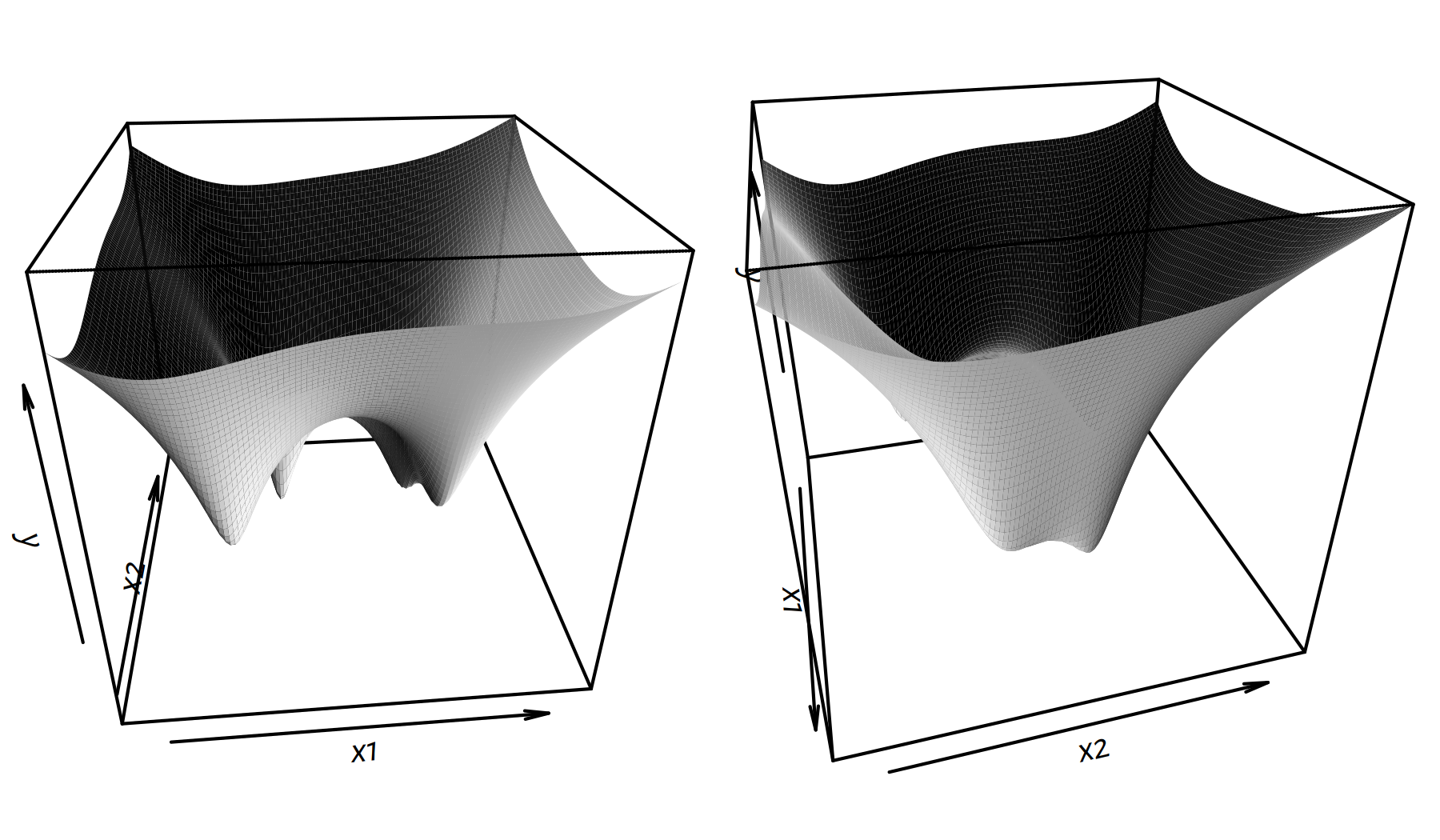
Figure 6.6: Perspective plots of \(g(x_1,x_2)\)
- Remark.
-
As usual, depicting functions that are defined over high-dimensional (3D and higher) domains is… difficult. Usually 1D or 2D projections can give us some neat intuitions though.
6.2 Iterative Methods
6.2.1 Introduction
Many optimisation algorithms are built around the following scheme:
Starting from a random point, perform a walk, in each step deciding where to go based on the idea of where the location of the minimum might be.
- Example.
-
Imagine we’re to cycle from Deakin University’s Burwood Campus to the CBD not knowing the route and with GPS disabled – we’ll have to ask many people along the way, but we’ll eventually (because most people are good) get to some CBD (say, in Perth).
More formally, we are interested in iterative algorithms that operate in a greedy-like manner:
\(\mathbf{x}^{(0)}\) – initial guess (e.g., generated at random)
for \(i=1,...,M\):
- \(\mathbf{x}^{(i)} = \mathbf{x}^{(i-1)}+\text{[guessed direction]}\)
- if \(|f(\mathbf{x}^{(i)})-f(\mathbf{x}^{(i-1)})| < \varepsilon\) break
return \(\mathbf{x}^{(i)}\) as result
Note that there are two stopping criteria, based on:
- \(M\) = maximum number of iterations,
- \(\varepsilon\) = tolerance, e.g, \(10^{-8}\).
6.2.2 Example in R
R has a built-in function, optim(), that provides an implementation
of (amongst others) the BFGS method
(proposed by Broyden, Fletcher, Goldfarb and Shanno in 1970).
- Remark.
-
(*) BFGS uses the assumption that the objective function is smooth – the [guessed direction] is determined by computing the (partial) derivatives (or their finite-difference approximations). However, they might work well even if this is not the case. We’ll be able to derive similar algorithms (called quasi-Newton ones) ourselves once we learn about Taylor series approximation by reading a book/taking a course on calculus.
Here, we shall use the BFGS as a black-box continuous optimisation method, i.e., without going into how it has been defined (in terms of our assumed math skills, it might be too early for this). Despite that, will still be able to point out a few interesting patterns.
optim(par, fn, method="BFGS")where:
par– an initial guess (a numeric vector of length \(p\))fn– an objective function to minimise (takes a vector of length \(p\) on input, returns a single number)
Let us minimise the \(g\) function defined above (the one with the 2D domain):
# g needs to be rewritten to accept a 2-ary vector
g_vectorised <- function(x12) g(x12[1], x12[2])
# random starting point with coordinates in [-5, 5]
(x12_init <- runif(2, -5, 5))
## [1] -2.1242 2.8831(res <- optim(x12_init, g_vectorised, method="BFGS"))## $par
## [1] -1.5423 2.1564
##
## $value
## [1] 1.4131e-12
##
## $counts
## function gradient
## 101 21
##
## $convergence
## [1] 0
##
## $message
## NULLNote that:
pargives the location of the local minimum found,valuegives the value of \(g\) atpar,convergenceof 0 is a successful one (we were able to satisfy the \(|f(\mathbf{x}^{(i)})-f(\mathbf{x}^{(i-1)})| < \varepsilon\) condition).
We can even depict the points that the algorithm is “visiting”, see Figure 6.7.
- Remark.
-
(*) Technically, the algorithm needs to evaluate a few more points in order to make the decision on where to go next (BFGS approximates the gradient and the Hessian matrix).
g_vectorised_plot <- function(x12) {
    points(x12[1], x12[2], col=2, pch=3) # draw
    g(x12[1], x12[2]) # return value
}
contour(x1, x2, y, nlevels=25)
res <- optim(x12_init, g_vectorised_plot, method="BFGS")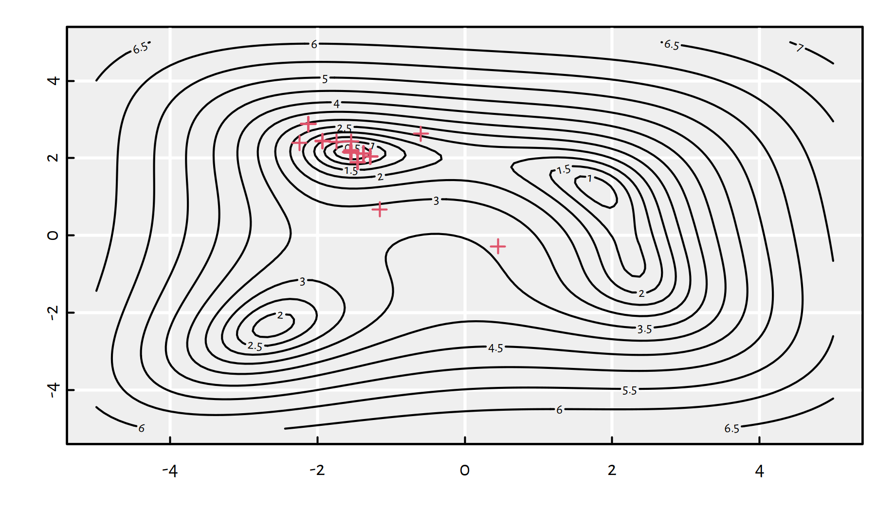
Figure 6.7: Each plotting symbol marks a point where the objective function was evaluated by the BFGS method
6.2.3 Convergence to Local Optima
We were lucky, because the local minimum that the algorithm has found coincides with the global minimum.
Let’s see where does the BFGS algorithm converge if seek the minimum of the above \(g\) starting from many randomly chosen points uniformly distributed over the square \([-5,5]\times[-5,5]\):
res_value <- replicate(1000, {
    # this will be iterated 100 times
    x12_init <- runif(2, -5, 5)
    res <- optim(x12_init, g_vectorised, method="BFGS")
    res$value # return value from each iteration
})
table(round(res_value,3))
##
## 0 0.695 1.356 1.705
## 273 352 156 219Unfortunately, we find the global minimum only in \(\sim 25\%\) cases, compare Figure 6.8.
hist(res_value, col="white", breaks=100, main=NA); box()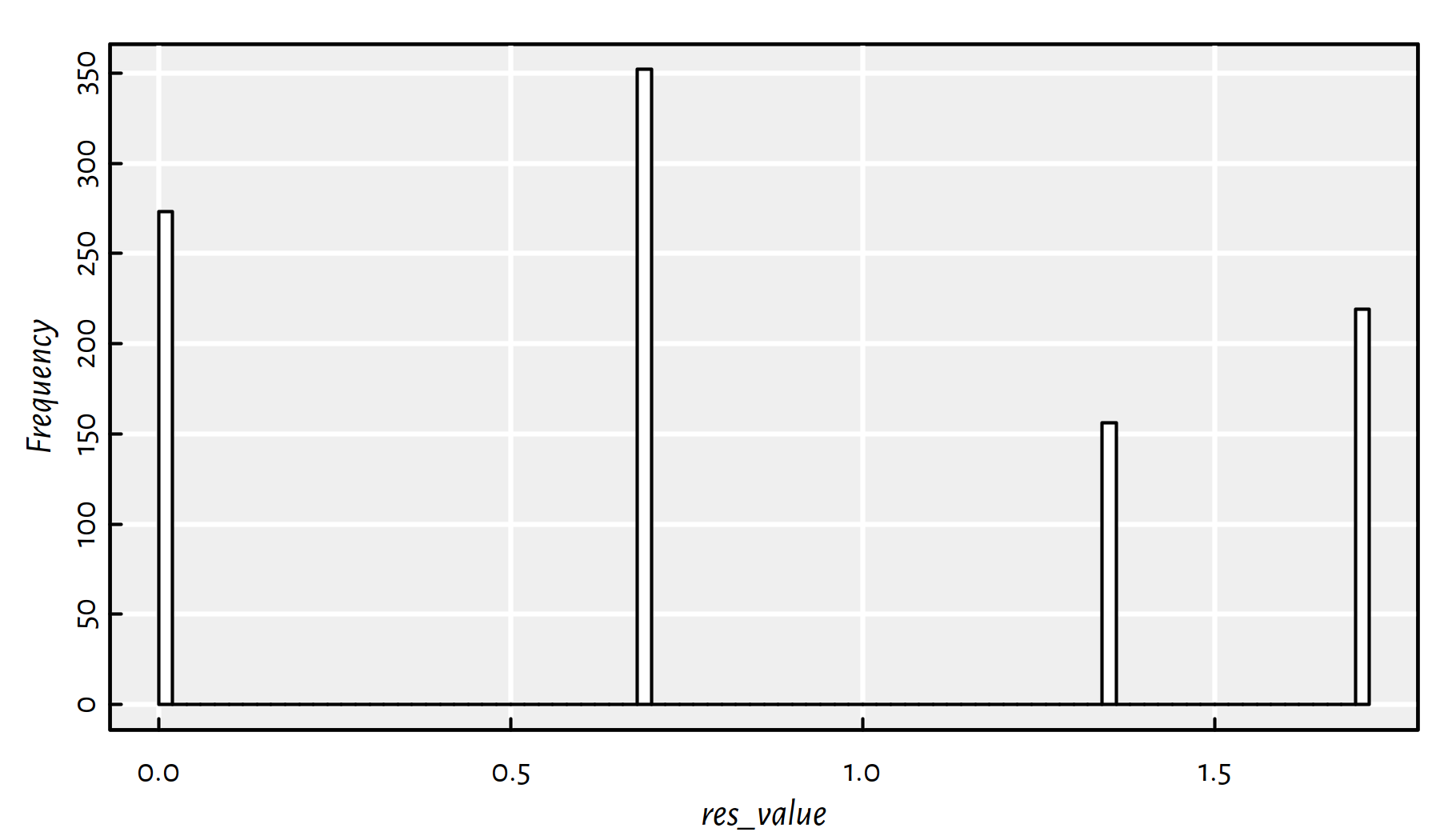
Figure 6.8: A histogram of the objective function’s value at the local minimum found when using a random initial guess
Figure 6.9 depicts all the random starting points and where do we converge from them.
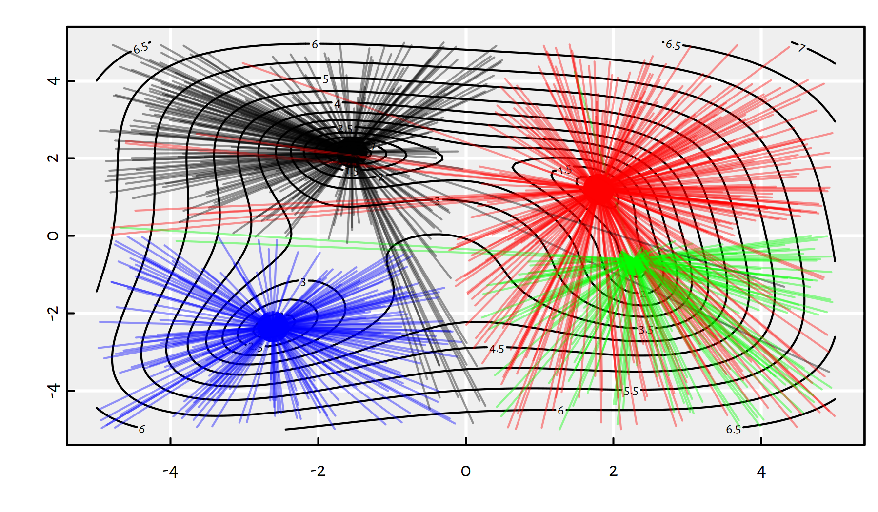
Figure 6.9: Each line segment connect a starting point to the point of BFGS’s convergence; note that by starting in the neighbourhood of \((0,-4)\) we can actually end up in any of the 4 local minima
6.2.4 Random Restarts
A kind of “remedy” for the above limitation could be provided by repeated local search: in order to robustify an optimisation procedure it is often advised to consider multiple random initial points and pick the best solution amongst the identified local optima.
# N             - number of restarts
# par_generator - a function generating initial guesses
# ...           - further arguments to optim()
optim_with_restarts <- function(par_generator, ..., N=10) {
    res_best <- list(value=Inf) # cannot be worse than this
    for (i in 1:N) {
        res <- optim(par_generator(), ...)
        if (res$value < res_best$value)
            res_best <- res # a better candidate found
    }
    res_best
}optim_with_restarts(function() runif(2, -5, 5),
g_vectorised, method="BFGS", N=10)## $par
## [1] -1.5423 2.1564
##
## $value
## [1] 3.9702e-13
##
## $counts
## function gradient
## 48 17
##
## $convergence
## [1] 0
##
## $message
## NULLFood for thought: Can we really really guarantee that the global minimum will be found within \(N\) tries?
Click here for a solution.
Absolutely not.
6.3 Gradient Descent
6.3.1 Function Gradient (*)
How to choose the [guessed direction] in our iterative optimisation algorithm?
If we are minimising a smooth function, the simplest possible choice is to use the information included in the objective’s gradient, which provides us with the information about the direction where the function decreases the fastest.
- Definition.
-
(*) Gradient of \(f:\mathbb{R}^p\to\mathbb{R}\), denoted \(\nabla f:\mathbb{R}^p\to\mathbb{R}^p\), is the vector of all its partial derivatives, (\(\nabla\) – nabla symbol = differential operator) \[ \nabla f(\mathbf{x}) = \left[ \begin{array}{c} \displaystyle\frac{\partial f}{\partial x_1}(\mathbf{x})\\ \vdots\\ \displaystyle\frac{\partial f}{\partial x_p}(\mathbf{x}) \end{array} \right] \] If we have a function \(f(x_1,...,x_p)\), the partial derivative w.r.t. the \(i\)-th variable, denoted \(\frac{\partial f}{\partial x_i}\) is like an ordinary derivative w.r.t. \(x_i\) where \(x_1,...,x_{i-1},x_{i+1},...,x_p\) are assumed constant.
- Remark.
-
Function differentiation is an important concept – see how it’s referred to in, e.g., the
keraspackage manual at https://keras.rstudio.com/reference/fit.html.
Recall our \(g\) function defined above: \[ g(x_1,x_2)=\log\left((x_1^{2}+x_2-5)^{2}+(x_1+x_2^{2}-3)^{2}+x_1^2-1.60644\dots\right) \]
It can be shown (*) that: \[ \begin{array}{ll} \frac{\partial g}{\partial x_1}(x_1,x_2)=& \displaystyle\frac{ 4x_1(x_1^{2}+x_2-5)+2(x_1+x_2^{2}-3)+2x_1 }{(x_1^{2}+x_2-5)^{2}+(x_1+x_2^{2}-3)^{2}+x_1^2-1.60644\dots} \\ \frac{\partial g}{\partial x_2}(x_1,x_2)=& \displaystyle\frac{ 2(x_1^{2}+x_2-5)+4x_2(x_1+x_2^{2}-3) }{(x_1^{2}+x_2-5)^{2}+(x_1+x_2^{2}-3)^{2}+x_1^2-1.60644\dots} \end{array} \]
grad_g_vectorised <- function(x) {
    c(
        4*x[1]*(x[1]^2+x[2]-5)+2*(x[1]+x[2]^2-3)+2*x[1],
        2*(x[1]^2+x[2]-5)+4*x[2]*(x[1]+x[2]^2-3)
    )/(
        (x[1]^2+x[2]-5)^2+(x[1]+x[2]^2-3)^2+x[1]^2-1.60644366086443841
    )
}
6.3.2 Three Facts on the Gradient
For now, we should emphasise three important facts:
- Fact 1.
-
If we are incapable of deriving the gradient analytically, we can rely on its finite differences approximation. Each partial derivative can be estimated by means of: \[ \frac{\partial f}{\partial x_i}(x_1,\dots,x_p) \simeq \frac{ f(x_1,...,x_i+\delta,...,x_p)-f(x_1,...,x_i,...,x_p) }{ \delta } \] for some small \(\delta>0\), say, \(\delta=10^{-6}\).
- Remark.
-
(*) Actually, a function’s partial derivative, by definition, is the limit of the above as \(\delta\to 0\).
Example implementation:
# gradient of f at x=c(x[1],...,x[p])
grad_approx <- function(f, x, delta=1e-6) {
    p <- length(x)
    gf <- numeric(p) # vector of length p
    for (i in 1:p) {
        xi <- x
        xi[i] <- xi[i]+delta
        gf[i] <- f(xi)
    }
    (gf-f(x))/delta
}- Remark.
-
(*) Interestingly, some modern vector/matrix algebra frameworks like TensorFlow (upon which
kerasis built) or PyTorch, feature methods to “derive” the gradient algorithmically (autodiff; automatic differentiation).
Sanity check:
grad_approx(g_vectorised, c(-2, 2))## [1] -3.1865 -1.3656grad_g_vectorised(c(-2, 2))## [1] -3.1865 -1.3656grad_approx(g_vectorised, c(-1.542255693, 2.15640528979))## [1] 1.0588e-05 1.9817e-05grad_g_vectorised(c(-1.542255693, 2.15640528979))## [1] 4.1292e-09 3.5771e-10By the way, there is also the grad() function in package numDeriv
that might be a little more accurate (uses a different approximation
formula).
- Fact 2.
-
The gradient of \(f\) at \(\mathbf{x}\), \(\nabla f(\mathbf{x})\), is a vector that points in the direction of the steepest slope. On the other hand, minus gradient, \(-\nabla f(\mathbf{x})\), is the direction where the function decreases the fastest.
- Remark.
-
(*) This can be shown by considering a function’s first-order Taylor series approximation.
Each gradient is a vector, therefore it can be depicted as an arrow. Figure 6.10 illustrates a few scaled gradients of the \(g\) function at different points – each arrow connects a point \(\mathbf{x}\) to \(\mathbf{x}\pm 0.1\nabla f(\mathbf{x})\).
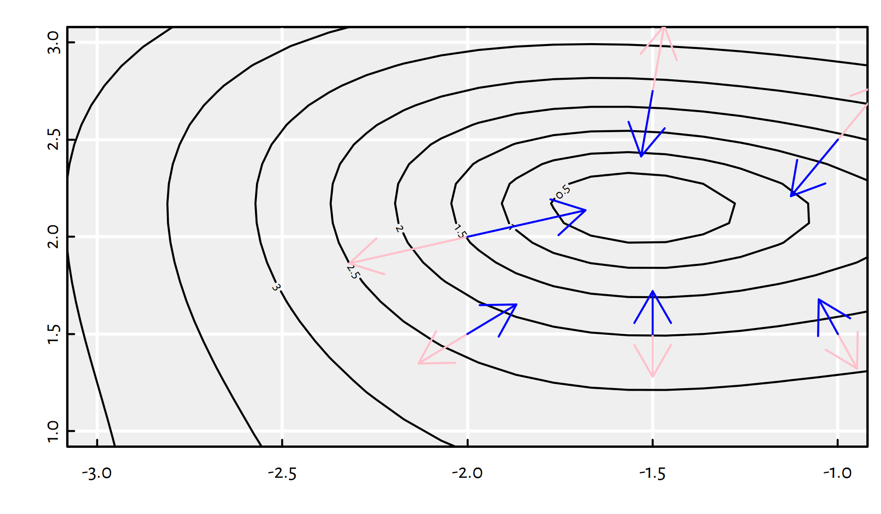
Figure 6.10: Scaled radients (pink arrows) and minus gradients (blue arrows) of \(g(x_1,x_2)\) at different points
Note that the blue arrows point more or less in the direction of the local minimum. Therefore, in our iterative algorithm, we may try taking the direction of the minus gradient! How far should we go in that direction? Well, a bit. We will refer to the desired step size as the learning rate, \(\eta\).
This will be called the gradient descent method (GD; Cauchy, 1847).
- Fact 3.
-
If a function \(f\) has a local minimum at \(\mathbf{x}^*\), then its gradient vanishes there, i.e., \(\nabla {f}(\mathbf{x}^*)=[0,\dots,0]\).
Note that the above condition is a necessary, not sufficient one. For example, the gradient also vanishes at a maximum or at a saddle point. In fact, we have what follows.
- Theorem.
-
(***) More generally, a twice-differentiable function has a local minimum at \(\mathbf{x}^*\) if and only if its gradient vanishes there and \(\nabla^2 {f}(\mathbf{x}^*)\) (Hessian matrix = matrix of all second-order derivatives) is positive-definite.
6.3.3 Gradient Descent Algorithm (GD)
Taking the above into account, we arrive at the gradient descent algorithm:
\(\mathbf{x}^{(0)}\) – initial guess (e.g., generated at random)
for \(i=1,...,M\):
- \(\mathbf{x}^{(i)} = \mathbf{x}^{(i-1)}-\eta \nabla f(\mathbf{x}^{(i-1)})\)
- if \(|f(\mathbf{x}^{(i)})-f(\mathbf{x}^{(i-1)})| < \varepsilon\) break
return \(\mathbf{x}^{(i)}\) as result
where \(\eta>0\) is a step size frequently referred to as the learning rate, because that’s much more cool. We usually set \(\eta\) of small order of magnitude, say \(0.01\) or \(0.1\).
An implementation of the gradient descent algorithm is straightforward.
In essence, it’s the par <- par - eta*grad_g_vectorised(par) expression
run in a loop, until convergence.
# par   - initial guess
# fn    - a function to be minimised
# gr    - a function to return the gradient of fn
# eta   - learning rate
# maxit - maximum number of iterations
# tol   - convergence tolerance
optim_gd <- function(par, fn, gr, eta=0.01,
                        maxit=1000, tol=1e-8) {
    f_last <- fn(par)
    for (i in 1:maxit) {
        par <- par - eta*grad_g_vectorised(par) # update step
        f_cur <- fn(par)
        if (abs(f_cur-f_last) < tol) break
        f_last <- f_cur
    }
    list( # see ?optim, section `Value`
        par=par,
        value=g_vectorised(par),
        counts=i,
        convergence=as.integer(i==maxit)
    )
}
Tests of the \(g\) function. First, let’s try \(\eta=0.01\). Figure 6.11 zooms in the contour plot so that we can see the actual path the algorithm has taken.
eta <- 0.01
res <- optim_gd(c(-3, 1), g_vectorised, grad_g_vectorised, eta=eta)
str(res)
## List of 4
## $ par : num [1:2] -1.54 2.16
## $ value : num 1.33e-08
## $ counts : int 135
## $ convergence: int 0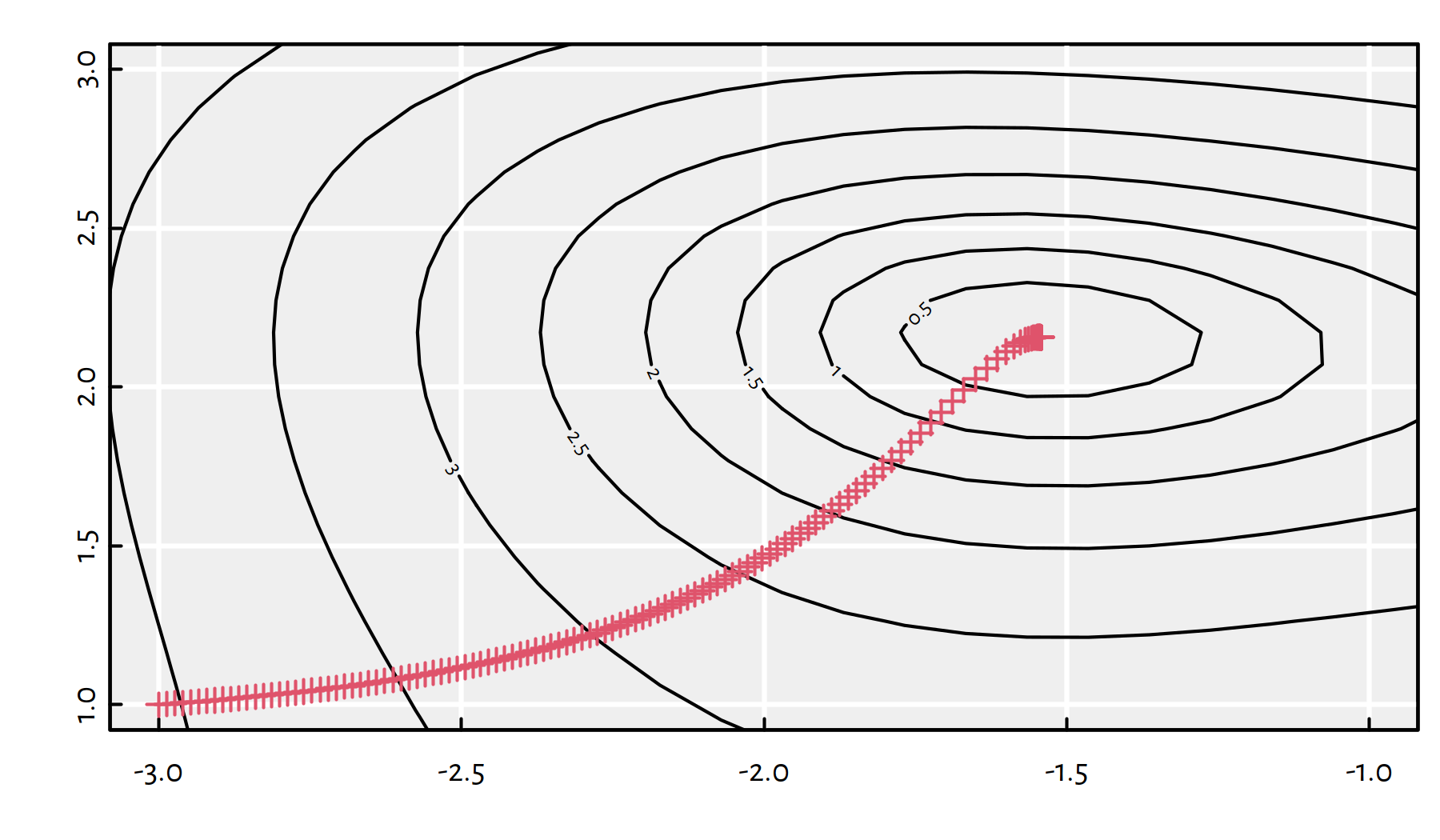
Figure 6.11: Path taken by the gradient descent algorithm with \(\eta=0.01\)
Now let’s try \(\eta=0.05\).
eta <- 0.05
res <- optim_gd(c(-3, 1), g_vectorised, grad_g_vectorised, eta=eta)
str(res)
## List of 4
## $ par : num [1:2] -1.54 2.15
## $ value : num 0.000203
## $ counts : int 417
## $ convergence: int 0With an increased step size, the algorithm needed many more iterations (3 times as many), see Figure 6.12 for the path taken.
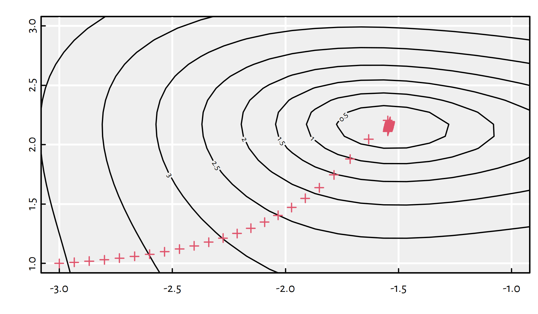
Figure 6.12: Path taken by the gradient descent algorithm with \(\eta=0.05\)
And now for something completely different: \(\eta=0.1\), see Figure 6.13.
eta <- 0.1
res <- optim_gd(c(-3, 1), g_vectorised, grad_g_vectorised, eta=eta)
str(res)
## List of 4
## $ par : num [1:2] -1.52 2.33
## $ value : num 0.507
## $ counts : int 1000
## $ convergence: int 1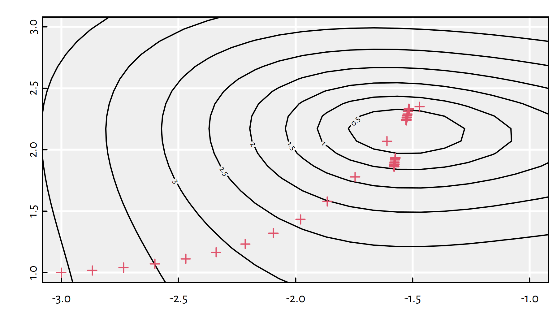
Figure 6.13: Path taken by the gradient descent algorithm with \(\eta=0.1\)
The algorithm failed to converge.
If the learning rate \(\eta\) is too small, the convergence might be too slow or we might get stuck at a plateau. On the other hand, if \(\eta\) is too large, we might be overshooting and end up bouncing around the minimum.
This is why many optimisation libraries (including keras/TensorFlow)
implement some
of the following ideas:
learning rate decay – start with large \(\eta\), decreasing it in every iteration, say, by some percent;
line search – determine optimal \(\eta\) in every step by solving a 1-dimensional optimisation problem w.r.t. \(\eta\in[0,\eta_{\max}]\);
momentum – the update step is based on a combination of the gradient direction and the previous change of the parameters, \(\Delta\mathbf{x}\); can be used to accelerate search in the relevant direction and minimise oscillations.
Try implementing at least the first of the above
heuristics yourself. You can set eta <- eta*0.95 in every iteration
of the gradient descent procedure.
6.3.4 Example: MNIST (*)
In the previous chapter we’ve studied the MNIST dataset. Let us go back to the task of fitting a multiclass logistic regression model.
library("keras")
mnist <- dataset_mnist()
## Loaded Tensorflow version 2.9.1# get train/test images in greyscale
X_train <- mnist$train$x/255 # to [0,1]
X_test <- mnist$test$x/255 # to [0,1]
# get the corresponding labels in {0,1,...,9}:
Y_train <- mnist$train$y
Y_test <- mnist$test$yThe labels need to be one-hot encoded:
one_hot_encode <- function(Y) {
    stopifnot(is.numeric(Y))
    c1 <- min(Y) # first class label
    cK <- max(Y) # last class label
    K <- cK-c1+1 # number of classes
    Y2 <- matrix(0, nrow=length(Y), ncol=K)
    Y2[cbind(1:length(Y), Y-c1+1)] <- 1
    Y2
}

Y_train2 <- one_hot_encode(Y_train)
Y_test2 <- one_hot_encode(Y_test)
Our task is to find the parameters \(\mathbf{B}\) that minimise cross entropy \(E(\mathbf{B})\) over the training set:
\[ \min_{\mathbf{B}\in\mathbb{R}^{785\times 10}} -\frac{1}{n^\text{train}} \sum_{i=1}^{n^\text{train}} \log \Pr(Y=y_i^\text{train}|\mathbf{x}_{i,\cdot}^\text{train},\mathbf{B}). \]
In the previous chapter, we’ve relied on the methods implemented
in the keras package. Let’s do that all by ourselves now.
In order to come up with a working version of the gradient
descent procedure for classifying of MNIST digits,
we will need to derive and implement grad_cross_entropy().
We do that below using matrix notation.
- Remark.
-
In the first reading, you can jump to the Safe landing zone below with no much loss in what we’re trying to convey here (you will then treat
grad_cross_entropy()as a black-box function). Nevertheless, keep in mind that this is the kind of maths you will need to master anyway sooner than later – this is inevitable. Perhaps you should go back to, e.g., the appendix on Matrix Computations with R or the chapter on Linear Regression? Learning maths is not a linear, step-by-step process. Everyone is different and will have a different path to success. The material needs to be frequently revisited, it will “click” someday, don’t you worry; good stuff isn’t built in a day or seven.
Recall that the output of the logistic regression model (1-layer neural network with softmax) can be written in the matrix form as: \[ \hat{\mathbf{Y}}=\mathrm{softmax}\left( \mathbf{\dot{X}}\,\mathbf{B} \right), \] where \(\mathbf{\dot{X}}\in\mathbb{R}^{n\times 785}\) is a matrix representing \(n\) images of size \(28\times 28\), augmented with a column of \(1\)s, and \(\mathbf{B}\in\mathbb{R}^{785\times 10}\) is the coefficients matrix and \(\mathrm{softmax}\) is applied on each matrix row separately.
Of course, by the definition of matrix multiplication, \(\hat{\mathbf{Y}}\) will be a matrix of size \(n\times 10\), where \(\hat{y}_{i,k}\) represents the predicted probability that the \(i\)-th image depicts the \(k\)-th digit.
# convert to matrices of size n*784
# and add a column of 1s
X_train1 <- cbind(1.0, matrix(X_train, ncol=28*28))
X_test1  <- cbind(1.0, matrix(X_test, ncol=28*28))
The nn_predict() function implements the above formula
for \(\hat{\mathbf{Y}}\):
softmax <- function(T) {
    T <- exp(T)
    T/rowSums(T)
}

nn_predict <- function(B, X) {
    softmax(X %*% B)
}
Let’s define the functions to compute the cross-entropy (which we shall minimise) and accuracy (which we shall report to a user):
cross_entropy <- function(Y_true, Y_pred) {
    -sum(Y_true*log(Y_pred))/nrow(Y_true)
}

accuracy <- function(Y_true, Y_pred) {
    # both arguments are one-hot encoded
    Y_true_decoded <- apply(Y_true, 1, which.max)
    Y_pred_decoded <- apply(Y_pred, 1, which.max)
    # proportion of equal corresponding pairs:
    mean(Y_true_decoded == Y_pred_decoded)
}
It may be shown (**) that the gradient of cross-entropy (with respect to the parameter matrix \(\mathbf{B}\)) can be expressed in the matrix form as:
\[ \frac{1}{n} \mathbf{\dot{X}}^T\, (\mathbf{\hat{Y}}-\mathbf{Y}) \]
grad_cross_entropy <- function(X, Y_true, Y_pred) {
    t(X) %*% (Y_pred-Y_true)/nrow(Y_true)
}
Of course, we could always substitute the gradient with the finite difference approximation. Yet, this would be much slower).
The more mathematically inclined reader will sure notice that by expanding the formulas given in the previous chapter, we can write cross-entropy in the non-matrix form (\(n\) – number of samples, \(K\) – number of classes, \(p+1\) – number of model parameters; in our case \(K=10\) and \(p=784\)) as:
\[ \begin{array}{rcl} E(\mathbf{B}) &=& -\displaystyle\frac{1}{n} \displaystyle\sum_{i=1}^n \displaystyle\sum_{k=1}^K y_{i,k} \log\left( \frac{ \exp\left( \displaystyle\sum_{j=0}^p \dot{x}_{i,j} \beta_{j,k} \right) }{ \displaystyle\sum_{c=1}^K \exp\left( \displaystyle\sum_{j=0}^p \dot{x}_{i,j} \beta_{j,c} \right) } \right)\\ &=& \displaystyle\frac{1}{n} \displaystyle\sum_{i=1}^n \left( \log \left(\displaystyle\sum_{k=1}^K \exp\left( \displaystyle\sum_{j=0}^p \dot{x}_{i,j} \beta_{j,k} \right)\right) - \displaystyle\sum_{k=1}^K y_{i,k} \displaystyle\sum_{j=0}^p \dot{x}_{i,j} \beta_{j,k} \right). \end{array} \]
Partial derivatives of cross-entropy w.r.t. \(\beta_{a,b}\) in non-matrix form can be derived (**) so as to get:
\[ \begin{array}{rcl} \displaystyle\frac{\partial E}{\partial \beta_{a,b}}(\mathbf{B}) &=& \displaystyle\frac{1}{n} \displaystyle\sum_{i=1}^n \dot{x}_{i,a} \left( \frac{ \exp\left( \displaystyle\sum_{j=0}^p \dot{x}_{i,j} \beta_{j,b} \right) }{ \displaystyle\sum_{k=1}^K \exp\left( \displaystyle\sum_{j=0}^p \dot{x}_{i,j} \beta_{j,k} \right) } - y_{i,b} \right)\\ &=& \displaystyle\frac{1}{n} \displaystyle\sum_{i=1}^n \dot{x}_{i,a} \left( \hat{y}_{i,b} - y_{i,b} \right). \end{array} \]
- Safe landing zone.
-
In case you’re lost with the above, continue from here. However, in the near future, harden up and revisit the skipped material to get the most out of our discussion.
We now have all the building blocks to
implement the gradient descent method.
The algorithm below follows exactly the same scheme as the one in the
\(g\) function example. This time, however, we play with a parameter matrix
\(\mathbf{B}\) (not a parameter vector \([x_1, x_2]\)) and we compute
the gradient of cross-entropy (by means of grad_cross_entropy()),
not the gradient of \(g\).
Note that a call to system.time(expr) measures the time (in seconds)
spent evaluating an expression expr.
# random matrix of size 785x10 - initial guess
B <- matrix(rnorm(ncol(X_train1)*ncol(Y_train2)),
    nrow=ncol(X_train1))
eta <- 0.1   # learning rate
maxit <- 100 # number of GD iterations
system.time({ # measure time spent
    # for simplicity, we stop only when we reach maxit
    for (i in 1:maxit) {
        B <- B - eta*grad_cross_entropy(
            X_train1, Y_train2, nn_predict(B, X_train1))
    }
}) # `user` - processing time in seconds:
## user system elapsed
## 90.573 39.037 32.149Unfortunately, the method’s convergence is really slow (we are optimising over \(7850\) parameters…) and the results after 100 iterations are disappointing:
accuracy(Y_train2, nn_predict(B, X_train1))## [1] 0.46462accuracy(Y_test2, nn_predict(B, X_test1))## [1] 0.4735Recall that in the previous chapter
we obtained much better classification accuracy by using the keras package.
What are we doing wrong then? Maybe keras implements some Super-Fancy
Hyper Optimisation Framework (TM) (R) that we could get access to for
only $19.99 per month?
6.3.5 Stochastic Gradient Descent (SGD) (*)
In turns out that there’s a very simple cure for the slow convergence of our method.
It might be shocking for some, but sometimes the true global minimum of cross-entropy for the whole training set is not exactly what we really want. In our predictive modelling task, we are minimising train error, but what we actually desire is to minimise the test error (which we cannot refer to while training = no cheating!).
It is therefore rational to assume that both the train and the test set consist of random digits independently sampled from the set of “all the possible digits out there in the world”.
Looking at the original objective (cross-entropy):
\[ E(\mathbf{B}) = -\frac{1}{n^\text{train}} \sum_{i=1}^{n^\text{train}} \log \Pr(Y=y_i^\text{train}|\mathbf{x}_{i,\cdot}^\text{train},\mathbf{B}). \]
How about we try fitting to different random samples of the train set in each iteration of the gradient descent method instead of fitting to the whole train set?
\[ E(\mathbf{B}) \simeq -\frac{1}{b} \sum_{i=1}^b \log \Pr(Y=y_{\text{random\_index}_i}^\text{train}|\mathbf{x}_{\text{random\_index}_i,\cdot}^\text{train},\mathbf{B}), \]
where \(b\) is some fixed batch size. Such an approach is often called stochastic gradient descent.
- Remark.
-
This scheme is sometimes referred to as mini-batch gradient descent in the literature; some researchers reserve the term “stochastic” only for batches of size 1.
Stochastic gradient descent can be implemented very easily:
B <- matrix(rnorm(ncol(X_train1)*ncol(Y_train2)),
    nrow=ncol(X_train1))
eta <- 0.1
maxit <- 100
batch_size <- 32
system.time({
    for (i in 1:maxit) {
        wh <- sample(nrow(X_train1), size=batch_size)
        B <- B - eta*grad_cross_entropy(
            X_train1[wh,], Y_train2[wh,],
            nn_predict(B, X_train1[wh,])
        )
    }
})
## user system elapsed
## 0.078 0.005 0.082accuracy(Y_train2, nn_predict(B, X_train1))## [1] 0.46198accuracy(Y_test2, nn_predict(B, X_test1))## [1] 0.4693The errors are much worse but at least we got the (useless) solution very quickly. That’s the “fail fast” rule in practice.
However, why don’t we increase the number of iterations and see what happens? We’ve allowed the classic gradient descent to scrabble around the MNIST dataset for almost 2 minutes.
B <- matrix(rnorm(ncol(X_train1)*ncol(Y_train2)),
    nrow=ncol(X_train1))
eta <- 0.1
maxit <- 10000
batch_size <- 32
system.time({
    for (i in 1:maxit) {
        wh <- sample(nrow(X_train1), size=batch_size)
        B <- B - eta*grad_cross_entropy(
            X_train1[wh,], Y_train2[wh,],
            nn_predict(B, X_train1[wh,])
        )
    }
})
## user system elapsed
## 7.312 0.140 7.453accuracy(Y_train2, nn_predict(B, X_train1))## [1] 0.89222accuracy(Y_test2, nn_predict(B, X_test1))## [1] 0.8935Bingo! Let’s take a closer look at how the train/test error
behaves in each iteration for different batch sizes.
Figures 6.14 and 6.15 depict
the cases of batch_size of 32 and 128, respectively.
The time needed to go through 10000 iterations with batch size of 32 is:
##    user  system elapsed
##  82.636  25.538  32.599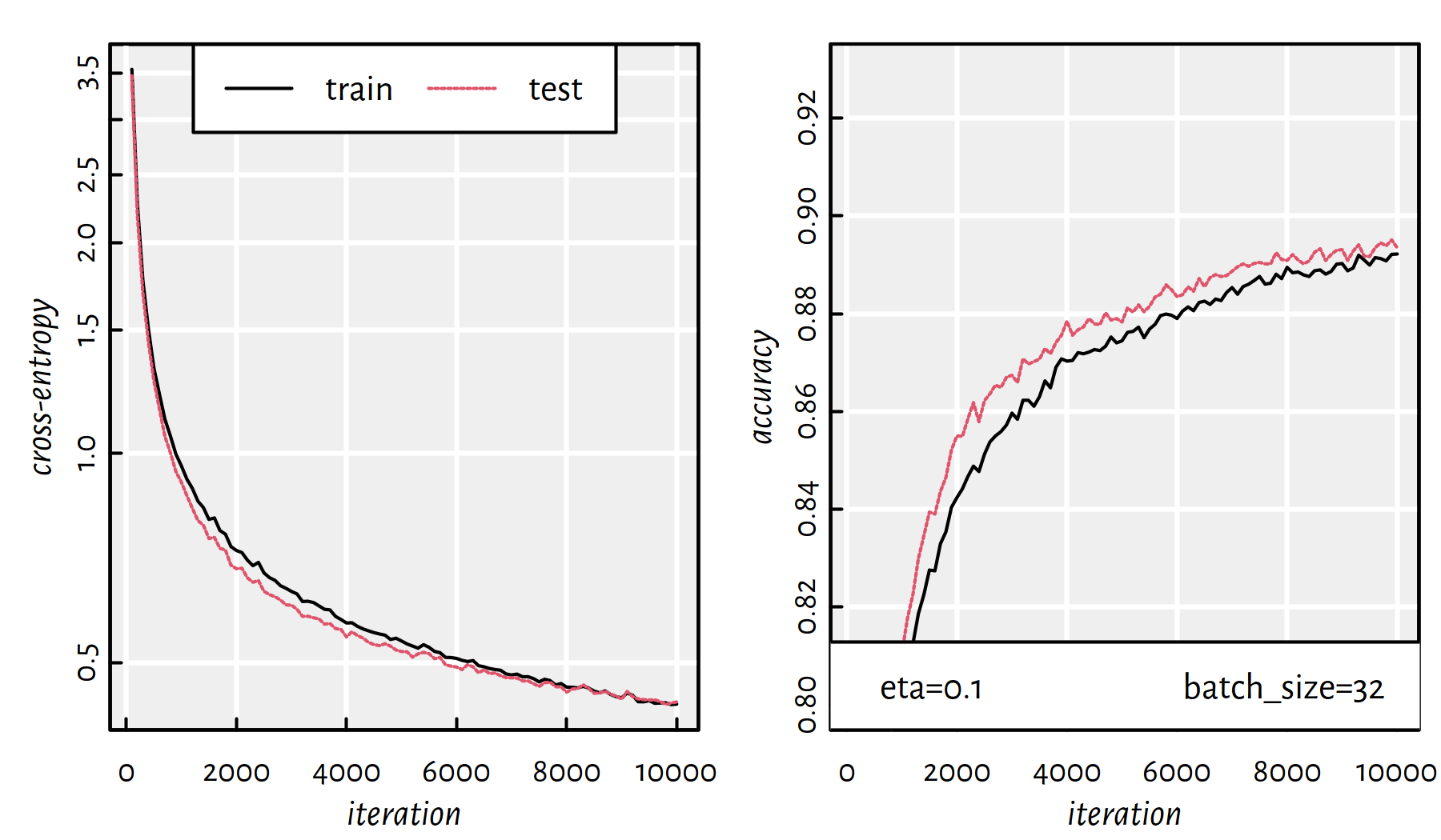
Figure 6.14: Cross-entropy and accuracy on the train and test set in each iteration of SGD; batch size of 32
What’s more, batch size of 128 takes:
##    user  system elapsed
## 198.066  93.369  56.396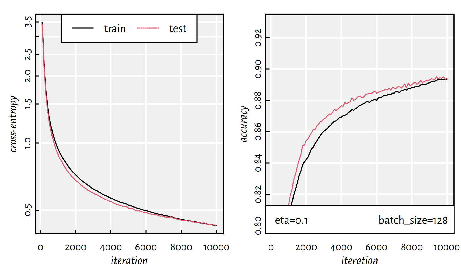
Figure 6.15: Cross-entropy and accuracy on the train and test set in each iteration of SGD; batch size of 128
Draw conclusions.
6.4 A Note on Convex Optimisation (*)
Are there any cases where we are sure that a local minimum is the global minimum? It turns out that the answer to this is positive; for example, when we minimise objective functions that fulfil a special property defined below.
First let’s note that given two points \(\mathbf{x}_{1},\mathbf{x}_{2}\in \mathbb{R}^p\), by taking any \(\theta\in[0,1]\), the point defined as:
\[ \mathbf{t} = \theta \mathbf{x}_{1}+(1-\theta)\mathbf{x}_{2} \]
lies on a (straight) line segment between \(\mathbf{x}_1\) and \(\mathbf{x}_2\).
- Definition.
-
We say that a function \(f:\mathbb{R}^p\to\mathbb{R}\) is convex, whenever: \[ (\forall \mathbf{x}_{1},\mathbf{x}_{2}\in \mathbb{R}^p) (\forall \theta\in [0,1])\quad f(\theta \mathbf{x}_{1}+(1-\theta)\mathbf{x}_{2})\leq \theta f(\mathbf{x}_{1})+(1-\theta)f(\mathbf{x}_{2}) \]
In other words, the function’s value at any convex combination of two points is not greater than that combination of the function values at these two points. See Figure 6.16 for a graphical illustration of the above.
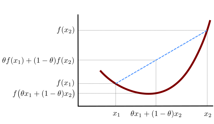
Figure 6.16: An illustration of the definition of a convex function
The following result addresses the question we posed at the beginning of this section.
- Theorem.
-
For any convex function \(f\), if \(f\) has a local minimum at \(\mathbf{x}^+\) then \(\mathbf{x}^+\) is also its global minimum.
Convex functions are ubiquitous in machine learning, but of course not every objective function we are going to deal with will fulfil this property. Here are some basic examples of convex functions and how they come into being, see, e.g., (Boyd & Vandenberghe 2004) for more:
- the functions mapping \(x\) to \(x, x^2, |x|, e^x\) are all convex,
- \(f(x)=|x|^p\) is convex for all \(p\ge 1\),
- if \(f\) is convex, then \(-f\) is concave,
- if \(f_1\) and \(f_2\) are convex, then \(w_1 f_1 + w_2 f_2\) are convex for any \(w_1,w_2\ge 0\),
- if \(f_1\) and \(f_2\) are convex, then \(\max\{f_1, f_2\}\) is convex,
- if \(f\) and \(g\) are convex and \(g\) is non-decreasing, then \(g(f(x))\) is convex.
The above feature the building blocks of our error measures in supervised learning problems! In particular, sum of squared residuals in linear regression is a convex function of the underlying parameters. Also, cross-entropy in logistic regression is a convex function of the underlying parameters.
- Theorem.
-
(***) If a function is twice differentiable, then its convexity can be judged based on the positive-definiteness of its Hessian matrix.
Note that optimising convex functions is relatively easy, especially if they are differentiable. This is because they are quite well-behaving. However, it doesn’t mean that we an analytic solution to the problem of their minimisation. Methods such as gradient descent or BFGS should work well (unless there are vast regions where a function is constant or the function’s is defined over a large number of parameters).
- Remark.
-
(**) There is a special class of constrained optimisation problems called linear and, more generally, quadratic programming that involves convex functions. Moreover, the Karush–Kuhn–Tucker (KKT) conditions address the more general problem of minimisation with constraints (i.e., not over the whole \(\mathbb{R}^p\) set); see (Nocedal & Wright 2006, Fletcher 2008) for more details.
- Remark.
-
Not only functions, but also sets can be said to be convex. We say that \(C\subseteq \mathbb{R}^p\) is a convex set, whenever the line segment joining any two points in \(C\) is fully included in \(C\). More formally, for every \(\mathbf{x}_1\in C\) and \(\mathbf{x}_2\in C\), it holds \(\theta \mathbf{x}_{1}+(1-\theta)\mathbf{x}_{2} \in C\) for all \(\theta\in [0,1]\); see Figure 6.17 for an illustration.
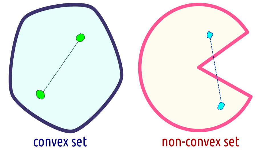
Figure 6.17: A convex and a non-convex set
6.5 Outro
6.5.1 Remarks
Solving continuous problems with many variables (e.g., deep neural networks) is time consuming – the more variables to optimise over (e.g., model parameters, think the number of interconnections between all the neurons), the slower the optimisation process.
Moreover, it might be the case that the sole objective function takes long to compute (think of image classification with large training samples).
- Remark.
-
(*) Although theoretically possible, good luck fitting a logistic regression model to MNIST with
optim()’s BFGS – there are 7850 variables!
Training deep neural networks with SGD is even slower (more parameters),
but there is a trick to propagate weight updates layer by layer,
called backpropagation (actually used in every neural network library),
see, e.g., (Sarle et al. 2002) and (Goodfellow et al. 2016).
Moreover, keras and similar libraries implement automatic differentiation
procedures that make its user’s life much easier (swiping some of the tedious
math under the comfy carpet).
keras implements various optimisers that
we can refer to in the compile() function,
see
https://keras.rstudio.com/reference/compile.html
and
https://keras.io/optimizers/:
SGD– stochastic gradient descent supporting momentum and learning rate decay,RMSprop– divides the gradient by a running average of its recent magnitude,Adam– adaptive momentum,
and so on. These are all non-complicated variations of the pure stochastic GD. Some of them are just tricks that work well in some examples and destroy the convergence on many other ones. You can get into their details in a dedicated book/course aimed at covering neural networks (see, e.g., (Sarle et al. 2002), (Goodfellow et al. 2016)), but we have already developed some good intuitions here.
Keep in mind that with methods such as GD or SGD, there is no guarantee we reach a minimum, but an approximate solution is better than no solution at all. Also sometimes (especially in ML applications) we don’t really need the actual minimum (e.g., when optimising the error with respect to the train set). Those “mathematically pure” will find that a bit… unaesthetic, but here we are. Maybe the solution makes your boss or client happy, maybe it generates revenue. Maybe it helps solve some other problem. Some claim that a solution is better than no solution at all, remember? But… is it really always the case though?
6.5.2 Further Reading
Recommended further reading: (Nocedal & Wright 2006), (Boyd & Vandenberghe 2004), (Fletcher 2008).