9 Recommender Systems (*)
These lecture notes are distributed in the hope that they will be useful. Any bug reports are appreciated.
9.1 Introduction
Recommender (recommendation) systems aim to predict the rating a user would give to an item.
For example:
- playlist generators (Spotify, YouTube, Netflix, …),
- content recommendations (Facebook, Instagram, Twitter, Apple News, …),
- product recommendations (Amazon, Alibaba, …).
Implementing recommender systems, according to (Ricci et al. 2011), might:
- increase the number of items sold,
- increase users’ satisfaction,
- increase users’ fidelity,
- allow a company to sell more diverse items,
- allow to better understand what users want.
Think of the last time you found some recommendation useful.
They can also increase the users’ frustration.
Think of the last time you found a recommendation useless and irritating. What might be the reasons why you have been provided with such a suggestion?
9.1.1 The Netflix Prize
In 2006 Netflix (back then a DVD rental company) released one of the most famous benchmark sets for recommender systems, which helped boost the research on algorithms in this field.
See https://www.kaggle.com/netflix-inc/netflix-prize-data; data archived at https://web.archive.org/web/20090925184737/http://archive.ics.uci.edu/ml/datasets/Netflix+Prize and https://archive.org/details/nf_prize_dataset.tar
The dataset consists of:
- 480,189 users
- 17,770 movies
- 100,480,507 ratings in the training sample:
MovieIDCustomerIDRatingfrom 1 to 5TitleYearOfReleasefrom 1890 to 2005Dateof rating in the range 1998-11-01 to 2005-12-31
The quiz set consists of 1,408,342 ratings and it was used by the competitors to assess the quality of their algorithms and compute the leaderboard scores.
Root mean squared error (RMSE) of predicted vs. true rankings was chosen as a performance metric.
The test set of 1,408,789 ratings (not make publicly available) was used to determine the winner.
On 21 September 2009, the grand prize of US$1,000,000 was given to the BellKor’s Pragmatic Chaos team which improved over the Netflix’s Cinematch algorithm by 10.06%, achieving the winning RMSE of 0.8567 on the test subset.
9.1.2 Main Approaches
Current recommender systems are quite complex and use a fusion of various approaches, also those based on external knowledge bases.
However, we may distinguish at least two core approaches, see (Ricci et al. 2011) for more:
Collaborative Filtering is based on the assumption that if two people interact with the same product, they’re likely to have other interests in common as well.
John and Mary both like bananas and apples and dislike spinach. John likes sushi. Mary hasn’t tried sushi yet. It seems they might have similar tastes, so we recommend that Mary should give sushi a try.
Content-based Filtering builds users’ profiles that represent information about what kind of products they like.
We have discovered that John likes fruit but dislikes vegetables. An orange is a fruit (an item similar to those he liked in the past) with which John is yet to interact. Thus, it is suggested that John should give it a try.
Jim Bennett, at that time the vice president of recommendation systems at Netflix on the idea behind the original Cinematch algorithm (see https://www.technologyreview.com/s/406637/the-1-million-netflix-challenge/ and https://web.archive.org/web/20070821194257/http://www.netflixprize.com/faq):
First, you collect 100 million user ratings for about 18,000 movies. Take any two movies and find the people who have rated both of them. Then look to see if the people who rate one of the movies highly rate the other one highly, if they liked one and not the other, or if they didn’t like either movie. Based on their ratings, Cinematch sees whether there’s a correlation between those people. Now, do this for all possible pairs of 65,000 movies.
Is the above an example of the collaborative or context-based filtering?
9.1.3 Formalism
Let \(\mathcal{U}=\{ U_1,\dots,U_n \}\) denote the set of \(n\) users.
Let \(\mathcal{I}=\{ I_1,\dots,I_p \}\) denote the set of \(p\) items.
Let \(\mathbf{R}\in\mathbb{R}^{n\times p}\) be a user-item matrix such that: \[ r_{u,i}=\left\{ \begin{array}{ll} r & \text{if the $u$-th user ranked the $i$-th item as $r>0$}\\ 0 & \text{if the $u$-th user hasn't interacted with the $i$-th item yet}\\ \end{array} \right. \]
- Remark.
-
Note that
0is used to denote a missing value (NA) here.
In particular, we can assume:
- \(r_{u,i}\in\{0,1,\dots,5\}\) (ratings on the scale 1–5 or no interaction)
- \(r_{u,i}\in\{0,1\}\) (“Like” or no interaction)
The aim of an recommender system is to predict the rating \(\hat{r}_{u,i}\) that the \(u\)-th user would give to the \(i\)-th item provided that currently \(r_{u,i}=0\).
9.2 Collaborative Filtering
9.2.1 Example
| . | Apple | Banana | Sushi | Spinach | Orange |
|---|---|---|---|---|---|
| Anne | 1 | 5 | 5 | 1 | |
| Beth | 1 | 1 | 5 | 5 | 1 |
| John | 5 | 5 | 1 | ||
| Kate | 1 | 1 | 5 | 5 | 1 |
| Mark | 5 | 5 | 1 | 1 | 5 |
| Sara | ? | 5 | ? | 5 |
In user-based collaborative filtering, we seek users with similar preference profiles/rating patters.
“User A has similar behavioural patterns as user B, so A should suggested with what B likes.”
In item-based collaborative filtering, we seek items with similar (dis)likeability structure.
“Users who (dis)liked X also (dis)liked Y”.
Will Sara enjoy her spinach? Will Sara enjoy her apple?
An example \(\mathbf{R}\) matrix in R:
R <- matrix(
    c(
     1, 5, 5, 0, 1,
     1, 1, 5, 5, 1,
     5, 5, 0, 1, 0,
     1, 1, 5, 5, 1,
     5, 5, 1, 1, 5,
     0, 5, 0, 0, 5
    ), byrow=TRUE, nrow=6, ncol=5,
    dimnames=list(
        c("Anne", "Beth", "John", "Kate", "Mark", "Sara"),
        c("Apple", "Banana", "Sushi", "Spinach", "Orange")
    )
)R## Apple Banana Sushi Spinach Orange
## Anne 1 5 5 0 1
## Beth 1 1 5 5 1
## John 5 5 0 1 0
## Kate 1 1 5 5 1
## Mark 5 5 1 1 5
## Sara 0 5 0 0 59.2.2 Similarity Measures
Assuming \(\mathbf{a},\mathbf{b}\) are two sequences of length \(k\) (in our setting, \(k\) is equal to either \(n\) or \(p\)), let \(S\) be the following similarity measure between two rating vectors:
\[ S(\mathbf{a},\mathbf{b}) = \frac{ \sum_{i=1}^k a_i b_i }{ \sqrt{ \sum_{i=1}^k a_i^2 } \sqrt{ \sum_{i=1}^k b_i^2 } } \]
cosim <- function(a, b) sum(a*b)/sqrt(sum(a^2)*sum(b^2))We call it the cosine similarity. We have \(S(\mathbf{a},\mathbf{b})\in[-1,1]\), where we get \(1\) for two identical elements. Similarity of 0 is obtained for two unrelated (“orthogonal”) vectors. For nonnegative sequences, negative similarities are not generated.
(*) Another frequently considered similarity measure is a version of the Pearson correlation coefficient that ignores all \(0\)-valued observations, see also the
useargument to thecor()function.
9.2.3 User-Based Collaborative Filtering
User-based approaches involve comparing each user against every other user (pairwise comparisons of the rows in \(\mathbf{R}\)). This yields a similarity degree between the \(i\)-th and the \(j\)-th user:
\[ s^U_{i,j} = S(\mathbf{r}_{i,\cdot},\mathbf{r}_{j,\cdot}). \]
SU <- matrix(0, nrow=nrow(R), ncol=nrow(R),
    dimnames=dimnames(R)[c(1,1)]) # and empty n*n matrix
for (i in 1:nrow(R)) {
    for (j in 1:nrow(R)) {
        SU[i,j] <- cosim(R[i,], R[j,])
    }
}round(SU, 2)## Anne Beth John Kate Mark Sara
## Anne 1.00 0.61 0.58 0.61 0.63 0.59
## Beth 0.61 1.00 0.29 1.00 0.39 0.19
## John 0.58 0.29 1.00 0.29 0.81 0.50
## Kate 0.61 1.00 0.29 1.00 0.39 0.19
## Mark 0.63 0.39 0.81 0.39 1.00 0.81
## Sara 0.59 0.19 0.50 0.19 0.81 1.00In order to obtain the previously unobserved rating \(\hat{r}_{u,i}\) using the user-based approach, we typically look for the \(K\) most similar users and aggregate their corresponding scores (for some \(K\ge 1\)).
More formally, let \(\{U_{v_1},\dots,U_{v_K}\}\in\mathcal{U}\setminus\{U_u\}\) be the set of users maximising \(s^U_{u, v_1}, \dots, s^U_{u, v_K}\) and having \(r_{v_1, i},\dots,r_{v_K, i}>0\). Then: \[ \hat{r}_{u,i} = \frac{1}{K} \sum_{\ell=1}^K r_{v_\ell, i}. \]
- Remark.
- The arithmetic mean can be replaced with, e.g., the more or a weighted arithmetic mean where weights are proportional to \(s^U_{u, v_\ell}\)
This is very similar to the \(K\)-nearest neighbour heuristic!
K <- 2
(sim <- order(SU["Sara",], decreasing=TRUE))
## [1] 6 5 1 3 2 4# sim gives the indices of people in decreasing order
# of similarity to Sara:
dimnames(R)[[1]][sim] # the corresponding names## [1] "Sara" "Mark" "Anne" "John" "Beth" "Kate"# Remove those who haven't tried Spinach yet (including Sara):
sim <- sim[ R[sim, "Spinach"]>0 ]
dimnames(R)[[1]][sim]## [1] "Mark" "John" "Beth" "Kate"# aggregate the Spinach ratings of the K most similar people:
mean(R[sim[1:K], "Spinach"])## [1] 19.2.4 Item-Based Collaborative Filtering
Item-based schemes rely on pairwise comparisons between the items (columns in \(\mathbf{R}\)). Hence, a similarity degree between the \(i\)-th and the \(j\)-th item is given by:
\[ s^I_{i,j} = S(\mathbf{r}_{\cdot,i},\mathbf{r}_{\cdot,j}). \]
SI <- matrix(0, nrow=ncol(R), ncol=ncol(R),
    dimnames=dimnames(R)[c(2,2)]) # an empty p*p matrix
for (i in 1:ncol(R)) {
    for (j in 1:ncol(R)) {
        SI[i,j] <- cosim(R[,i], R[,j])
    }
}round(SI, 2)## Apple Banana Sushi Spinach Orange
## Apple 1.00 0.78 0.32 0.38 0.53
## Banana 0.78 1.00 0.45 0.27 0.78
## Sushi 0.32 0.45 1.00 0.81 0.32
## Spinach 0.38 0.27 0.81 1.00 0.29
## Orange 0.53 0.78 0.32 0.29 1.00In order to obtain the previously unobserved rating \(\hat{r}_{u,i}\) using the item-based approach, we typically look for the \(K\) most similar items and aggregate their corresponding scores (for some \(K\ge 1\))
More formally, let \(\{I_{j_1},\dots,I_{j_K}\}\in\mathcal{I}\setminus\{I_i\}\) be the set of items maximising \(s^I_{i, j_1}, \dots, s^I_{i, j_K}\) and having \(r_{u, j_1},\dots,r_{u, j_K}>0\). Then:
\[ \hat{r}_{u,i} = \frac{1}{K} \sum_{\ell=1}^K r_{u, j_\ell}. \]
- Remark.
- Similarly to the previous case, the arithmetic mean can be replaced with, e.g., the mode or a weighted arithmetic mean where weights are proportional to \(s^I_{i, j_\ell}\).
K <- 2
(sim <- order(SI["Apple",], decreasing=TRUE))
## [1] 1 2 5 4 3# sim gives the indices of items in decreasing order
# of similarity to Apple:
dimnames(R)[[2]][sim] # the corresponding item types## [1] "Apple" "Banana" "Orange" "Spinach" "Sushi"# Remove these which Sara haven't tried yet (e.g., Apples):
sim <- sim[ R["Sara", sim]>0 ]
dimnames(R)[[2]][sim]## [1] "Banana" "Orange"# aggregate Sara's ratings of the K most similar items:
mean(R["Sara", sim[1:K]])## [1] 59.3 Exercise: The MovieLens Dataset (*)
9.3.1 Dataset
Let’s make a few recommendations based on the MovieLens-9/2018-Small dataset available at https://grouplens.org/datasets/movielens/latest/, see also https://movielens.org/ and (Harper & Konstan 2015).
The dataset consists of ca. 100,000 ratings to 9,000 movies by 600 users. It was last updated on September 2018.
This is already a pretty large dataset! We might run into problems with memory usage and high run-time.
movies <- read.csv("datasets/ml-9-2018-small/movies.csv",
    comment.char="#")
head(movies, 4)
## movieId title
## 1 1 Toy Story (1995)
## 2 2 Jumanji (1995)
## 3 3 Grumpier Old Men (1995)
## 4 4 Waiting to Exhale (1995)
## genres
## 1 Adventure|Animation|Children|Comedy|Fantasy
## 2 Adventure|Children|Fantasy
## 3 Comedy|Romance
## 4 Comedy|Drama|Romancenrow(movies)## [1] 9742ratings <- read.csv("datasets/ml-9-2018-small/ratings.csv",
comment.char="#")
head(ratings, 4)## userId movieId rating timestamp
## 1 1 1 4 964982703
## 2 1 3 4 964981247
## 3 1 6 4 964982224
## 4 1 47 5 964983815nrow(ratings)## [1] 100836table(ratings$rating)##
## 0.5 1 1.5 2 2.5 3 3.5 4 4.5 5
## 1370 2811 1791 7551 5550 20047 13136 26818 8551 132119.3.2 Data Cleansing
movieIds should be re-encoded, as not every film is mentioned/rated in the database.
We will re-map the movieIds to consecutive integers.
# the list of all rated movieIds:
movieId2 <- unique(ratings$movieId)
# max user Id (these could've been cleaned up too):
(n <- max(ratings$userId))
## [1] 610# number of unique movies:
(p <- length(movieId2))## [1] 9724# remove unrated movies:
movies <- movies[movies$movieId %in% movieId2, ]# we'll map movieId2[i] to i for each i=1,...,p:
movies$movieId <- match(movies$movieId, movieId2)
ratings$movieId <- match(ratings$movieId, movieId2)
# order the movies by the new movieId so that
# the movie with Id==i is in the i-th row:
movies <- movies[order(movies$movieId),]
stopifnot(all(movies$movieId == 1:p)) # sanity checkWe will use a sparse matrix data type (from R package Matrix)
to store the ratings data, \(\mathbf{R}\in\mathbb{R}^{n\times p}\).
- Remark.
- Sparse matrices contain many zeros. Instead of storing all the \(np=5931640\) elements, only the lists of non-zero ones are saved, \(100836\) values in total. This way, we might save a lot of memory. The drawback is that, amongst others, random access to the elements in a sparse matrix takes more time.
library("Matrix")
R <- Matrix(0.0, sparse=TRUE, nrow=n, ncol=p)
# This is a vectorised operation;
# it is faster than a for loop over each row
# in the ratings matrix:
R[cbind(ratings$userId, ratings$movieId)] <- ratings$rating
Let’s preview a few first rows and columns:
R[1:6, 1:18]## 6 x 18 sparse Matrix of class "dgCMatrix"
##
## [1,] 4 4 4 5 5 3 5 4 5 5 5 5 3 5 4 5 3 3
## [2,] . . . . . . . . . . . . . . . . . .
## [3,] . . . . . . . . . . . . . . . . . .
##
## ..............................
## ........suppressing 1 rows in show(); maybe adjust 'options(max.print= *, width = *)'
## ..............................
##
## [5,] 4 . . . 4 . . 4 . . . . . . . . 5 2
## [6,] . 5 4 4 1 . . 5 4 . 3 4 . 3 . . 2 59.3.3 Item-Item Similarities
To recall, the cosine similarity between \(\mathbf{r}_{\cdot,i},\mathbf{r}_{\cdot,j}\in\mathbb{R}^n\) is given by:
\[ s_{i,j}^I = S_C(\mathbf{r}_{\cdot,i},\mathbf{r}_{\cdot,j}) = \frac{\sum_{k=1}^n r_{k,i} \, r_{k,j}}{ \sqrt{\sum_{k=1}^n r_{k,i}^2}\sqrt{\sum_{k=1}^n r_{k,j}^2} } \]
In vector/matrix algebra notation, this is:
\[ s_{i,j}^I = S_C(\mathbf{r}_{\cdot,i},\mathbf{r}_{\cdot,j}) = \frac{\mathbf{r}_{\cdot,i}^T\, \mathbf{r}_{\cdot,j}}{ \sqrt{{\mathbf{r}_{\cdot,i}^T\, \mathbf{r}_{\cdot,i}}} \sqrt{{\mathbf{r}_{\cdot,j}^T\, \mathbf{r}_{\cdot,j}}} } \]
As \(\mathbf{R}\in\mathbb{R}^{n\times p}\), we can “almost” compute all the \(p\times p\) cosine similarities at once by applying:
\[ \mathbf{S}^I = \frac{\mathbf{R}^T \mathbf{R}}{ \dots } \]
Cosine similarities for item-item comparisons:
norms <- as.matrix(sqrt(colSums(R^2)))
Rx <- as.matrix(crossprod(R, R))
SI <- Rx/tcrossprod(norms)
SI[is.nan(SI)] <- 0 # there were some divisions by zero- Remark.
-
crossprod(A,B)gives \(\mathbf{A}^T \mathbf{B}\) andtcrossprod(A,B)gives \(\mathbf{A} \mathbf{B}^T\).
9.3.4 Example Recommendations
recommend <- function(i, K, SI, movies) {
    # get K most similar movies to the i-th one
    ms <- order(SI[i,], decreasing=TRUE)
    data.frame(
        Title=movies$title[ms[1:K]],
        SIC=SI[i,ms[1:K]]
    )
}movies$title[1215]## [1] "Monty Python's The Meaning of Life (1983)"recommend(1215, 10, SI, movies)## Title SIC
## 1 Monty Python's The Meaning of Life (1983) 1.00000
## 2 Monty Python's Life of Brian (1979) 0.61097
## 3 Monty Python and the Holy Grail (1975) 0.51415
## 4 House of Flying Daggers (Shi mian mai fu) (2004) 0.49322
## 5 Hitchhiker's Guide to the Galaxy, The (2005) 0.45482
## 6 Bowling for Columbine (2002) 0.45051
## 7 Shaun of the Dead (2004) 0.44566
## 8 O Brother, Where Art Thou? (2000) 0.44541
## 9 Ghost World (2001) 0.44416
## 10 Full Metal Jacket (1987) 0.44285movies$title[1]## [1] "Toy Story (1995)"recommend(1, 10, SI, movies)## Title SIC
## 1 Toy Story (1995) 1.00000
## 2 Toy Story 2 (1999) 0.57260
## 3 Jurassic Park (1993) 0.56564
## 4 Independence Day (a.k.a. ID4) (1996) 0.56426
## 5 Star Wars: Episode IV - A New Hope (1977) 0.55739
## 6 Forrest Gump (1994) 0.54710
## 7 Lion King, The (1994) 0.54115
## 8 Star Wars: Episode VI - Return of the Jedi (1983) 0.54109
## 9 Mission: Impossible (1996) 0.53891
## 10 Groundhog Day (1993) 0.53417…and so on.
9.3.5 Clustering
All our ratings are \(r_{i,j}\ge 0\), therefore the cosine similarity is \(s_{i,j}^I\ge 0\). Moreover, it holds \(s_{i,j}^I\le 1\). Thus, a cosine similarity matrix can be turned into a dissimilarity matrix:
DI <- 1.0-SI
DI[DI<0] <- 0.0 # account for numeric inaccuracies
DI <- as.dist(DI)
This enables us to perform, e.g., the cluster analysis of items:
library("genie")## Loading required package: genieclusth <- hclust2(DI)
plot(h, labels=FALSE, ann=FALSE); box()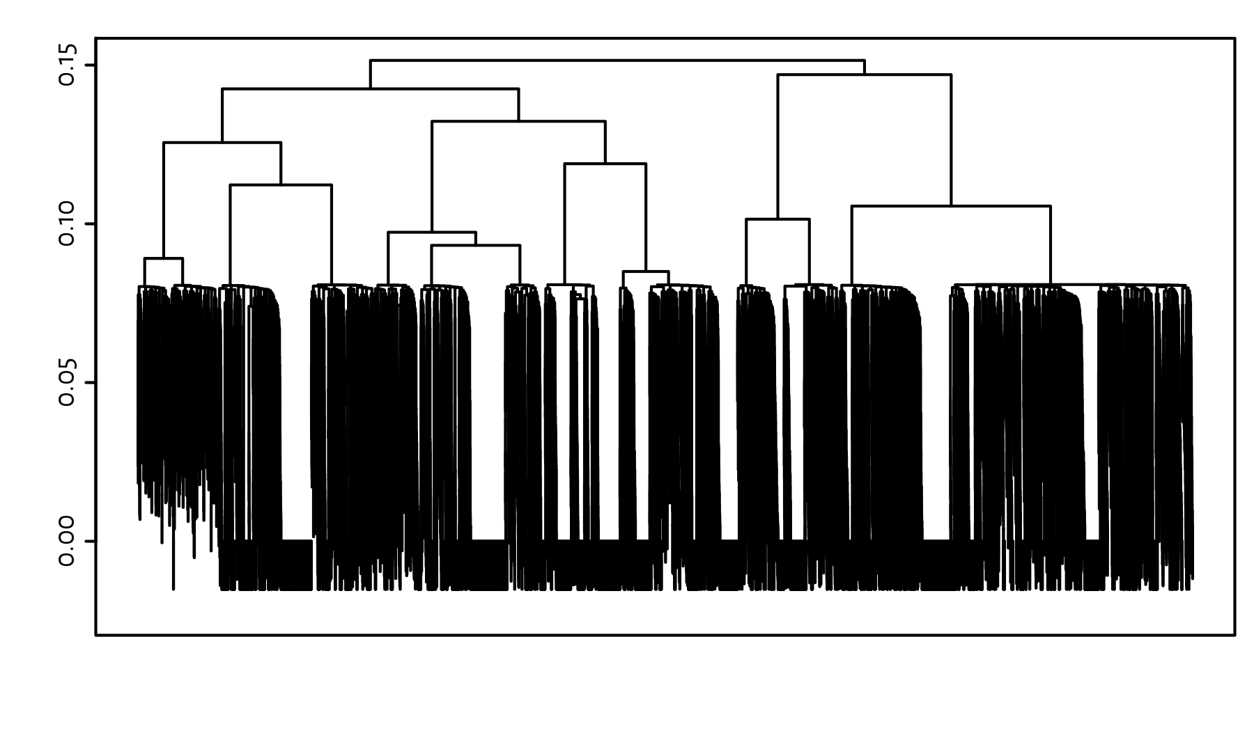
Figure 9.1: Cluster dendrogram for the movies
A 14-partition might look nice, let’s give it a try:
c <- cutree(h, k=14)Example movies in the 3rd cluster:
Bottle Rocket (1996), Clerks (1994), Star Wars: Episode IV - A New Hope (1977), Swingers (1996), Monty Python’s Life of Brian (1979), E.T. the Extra-Terrestrial (1982), Monty Python and the Holy Grail (1975), Star Wars: Episode V - The Empire Strikes Back (1980), Princess Bride, The (1987), Raiders of the Lost Ark (Indiana Jones and the Raiders of the Lost Ark) (1981), Star Wars: Episode VI - Return of the Jedi (1983), Blues Brothers, The (1980), Duck Soup (1933), Groundhog Day (1993), Back to the Future (1985), Young Frankenstein (1974), Indiana Jones and the Last Crusade (1989), Grosse Pointe Blank (1997), Austin Powers: International Man of Mystery (1997), Men in Black (a.k.a. MIB) (1997)
The definitely have something in common!
Example movies in the 1st cluster:
Toy Story (1995), Heat (1995), Seven (a.k.a. Se7en) (1995), Usual Suspects, The (1995), From Dusk Till Dawn (1996), Braveheart (1995), Rob Roy (1995), Desperado (1995), Billy Madison (1995), Dumb & Dumber (Dumb and Dumber) (1994), Ed Wood (1994), Pulp Fiction (1994), Stargate (1994), Tommy Boy (1995), Clear and Present Danger (1994), Forrest Gump (1994), Jungle Book, The (1994), Mask, The (1994), Fugitive, The (1993), Jurassic Park (1993)
… and so forth.
9.4 Outro
9.4.1 Remarks
Good recommender systems are perfect tools to increase the revenue of any user-centric enterprise.
Not a single algorithm, but an ensemble (a proper combination) of different approaches is often used in practice, see the Further Reading section below for the detailed information of the Netflix Prize winners.
Recommender systems are an interesting fusion of the techniques we have already studied – linear models, K-nearest neighbours etc.
Building recommender systems is challenging, because data is large yet often sparse. For instance, the ratio of available ratings vs. all possible user-item valuations for the Netflix Prize (obviously, it is just a sample of the complete dataset that Netflix has) is equal to:
100480507/(480189*17770)## [1] 0.011776A sparse matrix (see R package Matrix) data structure is
often used for storing of and computing over such data effectively.
Note that some users are biased in the sense that they are more critical or enthusiastic than average users.
Is 3 stars a “bad”, “fair enough” or “good” rating for you? Would you go to a bar/restaurant ranked 3.0 by you favourite Maps app community?
It is particularly challenging to predict the preferences of users that cast few ratings, e.g., those who just signed up (the cold start problem).
“Hill et al. [1995] have shown that users provide inconsistent ratings when asked to rate the same movie at different times. They suggest that an algorithm cannot be more accurate than the variance in a user’s ratings for the same item.” (Herlocker et al. 2004: p. 6)
It is good to take into account the temporal (time-based) characteristics of data as well as external knowledge (e.g., how long ago a rating was cast, what is a film’s genre).
The presented approaches are vulnerable to attacks – bots may be used to promote or inhibit selected items.
9.4.2 Further Reading
Recommended further reading:
(Herlocker et al. 2004),
(Ricci et al. 2011),
(Lü et al. 2012),
(Harper & Konstan 2015).
See also the Netflix prize winners: (Koren 2009),
(Töscher et al. 2009),
(Piotte & Chabbert 2009).
Also don’t forget to take a look at
the R package recommenderlab (amongst others).