8 Optimisation with Genetic Algorithms (*)

8.1.1 Recap

Recall that an optimisation task deals with finding an element \(\mathbf{x}\) in a search space \(\mathbb{D}\), that minimises or maximises an objective function \(f:\mathbb{D}\to\mathbb{R}\): \[ \min_{\mathbf{x}\in \mathbb{D}} f(\mathbf{x}) \quad\text{or}\quad\max_{\mathbf{x}\in \mathbb{D}} f(\mathbf{x}), \]

In one of the previous chapters, we were dealing with unconstrained continuous optimisation, i.e., we assumed the search space is \(\mathbb{D}=\mathbb{R}^p\) for some \(p\).

Example problems of this kind: minimising mean squared error in linear regression or minimising cross-entropy in logistic regression.

The class of general-purpose iterative algorithms we’ve previously studied fit into the following scheme:

1. \(\mathbf{x}^{(0)}\) – initial guess (e.g., generated at random)

2. for \(i=1,...,M\):

   1. \(\mathbf{x}^{(i)} = \mathbf{x}^{(i-1)}+\text{[guessed direction, e.g.,}-\eta\nabla f(\mathbf{x})\text{]}\)
   2. if \(|f(\mathbf{x}^{(i)})-f(\mathbf{x}^{(i-1)})| < \varepsilon\) break

3. return \(\mathbf{x}^{(i)}\) as result

where:

• \(M\) = maximum number of iterations
• \(\varepsilon\) = tolerance, e.g, \(10^{-8}\)
• \(\eta>0\) = learning rate

The algorithms such as gradient descent and BFGS (see optim()) give satisfactory results in the case of smooth and well-behaving objective functions.

However, if an objective has, e.g., many plateaus (regions where it is almost constant), those methods might easily get stuck in local minima.

The K-means clustering’s objective function is a not particularly pleasant one – it involves a nested search for the closest cluster, with the use of the \(\min\) operator.

8.1.2 K-means Revisited

In K-means clustering we are minimising the squared Euclidean distance to each point’s cluster centre: \[ \min_{\boldsymbol\mu_{1,\cdot}, \dots, \boldsymbol\mu_{K,\cdot} \in \mathbb{R}^p} \sum_{i=1}^n \left( \min_{k=1,\dots,K} \sum_{j=1}^p \left(x_{i,j}-\mu_{k,j}\right)^2 \right). \]

This is an (NP-)hard problem! There is no efficient exact algorithm.

We need approximations. In the last chapter, we have discussed the iterative Lloyd’s algorithm (1957), which is amongst a few procedures implemented in the kmeans() function.

To recall, Lloyd’s algorithm (1957) is sometimes referred to as “the” K-means algorithm:

1. Start with random cluster centres \(\boldsymbol\mu_{1,\cdot}, \dots, \boldsymbol\mu_{K,\cdot}\).

2. For each point \(\mathbf{x}_{i,\cdot}\), determine its closest centre \(C(i)\in\{1,\dots,K\}\).

3. For each cluster \(k\in\{1,\dots,K\}\), compute the new cluster centre \(\boldsymbol\mu_{k,\cdot}\) as the componentwise arithmetic mean of the coordinates of all the point indices \(i\) such that \(C(i)=k\).

4. If the cluster centres changed since last iteration, go to step 2, otherwise stop and return the result.

As the procedure might get stuck in a local minimum, a few restarts are recommended (as usual).

Hence, we are used to calling:

kmeans(X, centers=k, nstart=10)

8.1.3 optim() vs. kmeans()

Let us compare how a general-purpose optimiser such as the BFGS algorithm implemented in optim() compares with a customised, problem-specific solver.

We will need some benchmark data.

gen_cluster <- function(n, p, m, s) {
    vectors <- matrix(rnorm(n*p), nrow=n, ncol=p)
    unit_vectors <- vectors/sqrt(rowSums(vectors^2))
    unit_vectors*rnorm(n, 0, s)+rep(m, each=n)
}

The above function generates \(n\) points in \(\mathbb{R}^p\) from a distribution centred at \(\mathbf{m}\in\mathbb{R}^p\), spread randomly in every possible direction with scale factor \(s\).

Two example clusters in \(\mathbb{R}^2\):

# plot the "black" cluster
plot(gen_cluster(500, 2, c(0, 0), 1), col="#00000022", pch=16,
    xlim=c(-3, 4), ylim=c(-3, 4), asp=1, ann=FALSE)
# plot the "red" cluster
points(gen_cluster(250, 2, c(1.5, 1), 0.5), col="#ff000022", pch=16)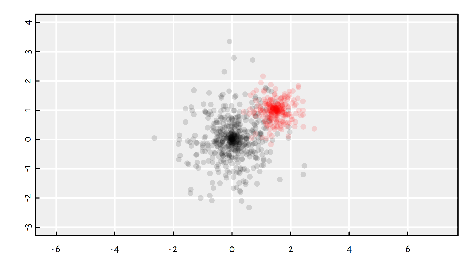

(#fig:gendata_example) plot of chunk gendata_example

Let’s generate the benchmark dataset \(\mathbf{X}\) that consists of three clusters in a high-dimensional space.

set.seed(123)
p  <- 32
Ns <- c(50, 100, 20)
Ms <- c(0, 1, 2)
s  <- 1.5*p
K  <- length(Ns)

X <- lapply(1:K, function(k)
    gen_cluster(Ns[k], p, rep(Ms[k], p), s))
X <- do.call(rbind, X) # rbind(X[[1]], X[[2]], X[[3]])

The objective function for the K-means clustering problem:

library("FNN")
get_loss <- function(mu, X) {
    # For each point in X,
    # get the index of the closest point in mu:
    memb <- FNN::get.knnx(mu, X, 1)$nn.index

    # compute the sum of squared distances
    # between each point and its closes cluster centre:
    sum((X-mu[memb,])^2)
}

Setting up the solvers:

min_HartiganWong <- function(mu0, X)
    get_loss(
        # algorithm="Hartigan-Wong"
        kmeans(X, mu0, iter.max=100)$centers,
    X)
min_Lloyd <- function(mu0, X)
    get_loss(
        kmeans(X, mu0, iter.max=100, algorithm="Lloyd")$centers,
    X)
min_optim <- function(mu0, X)
    optim(mu0,
        function(mu, X) {
            get_loss(matrix(mu, nrow=nrow(mu0)), X)
        }, X=X, method="BFGS", control=list(reltol=1e-16)
    )$val

Running the simulation:

nstart <- 100
set.seed(123)
res <- replicate(nstart, {
  mu0 <- X[sample(nrow(X), K),]
    c(
        HartiganWong=min_HartiganWong(mu0, X),
        Lloyd=min_Lloyd(mu0, X),
        optim=min_optim(mu0, X)
    )
})

Notice a considerable variability of the objective function at the local minima found:

boxplot(as.data.frame(t(res)), horizontal=TRUE, col="white")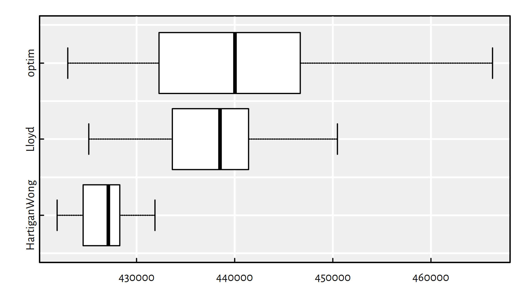

Figure 8.1: plot of chunk gendata5

print(apply(res, 1, function(x)
    c(summary(x), sd=sd(x))
))

##         HartiganWong    Lloyd  optim
## Min.          421889 425119.5 422989
## 1st Qu.       424663 433669.3 432446
## Median        427129 438502.2 440033
## Mean          426557 438075.0 440635
## 3rd Qu.       428243 441381.3 446614
## Max.          431869 450469.7 466303
## sd              2301   5709.3  10888

Of course, we are interested in the smallest value of the objective, because we’re trying to pinpoint the global minimum.

print(apply(res, 1, min))

## HartiganWong        Lloyd        optim 
##       421889       425119       422989

The Hartigan-Wong algorithm (the default one in kmeans()) is the most reliable one of the three:

• it gives the best solution (low bias)
• the solutions have the lowest degree of variability (low variance)
• it is the fastest:

library("microbenchmark")
set.seed(123)
mu0 <- X[sample(nrow(X), K),]
summary(microbenchmark(
    HartiganWong=min_HartiganWong(mu0, X),
    Lloyd=min_Lloyd(mu0, X),
    optim=min_optim(mu0, X),
    times=10
), unit="relative")

##           expr       min        lq      mean    median        uq
## 1 HartiganWong    1.0914    1.1464    1.1718    1.1764    1.2848
## 2        Lloyd    1.0000    1.0000    1.0000    1.0000    1.0000
## 3        optim 1611.1920 1606.1912 1537.1444 1591.3588 1570.4874
##         max neval
## 1    1.1449    10
## 2    1.0000    10
## 3 1316.5149    10

print(min(res))

## [1] 421889

Is it the global minimum?

We don’t know, we just didn’t happen to find anything better (yet).

Did we put enough effort to find it?

Well, maybe. We can try more random restarts:

res_tried_very_hard <- kmeans(X, K, nstart=100000, iter.max=10000)$centers
print(get_loss(res_tried_very_hard, X))

## [1] 421889

Is it good enough?

It depends what we’d like to do with this. Does it make your boss happy? Does it generate revenue? Does it help solve any other problem? Is it useful anyhow? Are you really looking for the global minimum?

8.2.1 Introduction

What if our optimisation problem cannot be solved reliably with gradient-based methods like those in optim() and we don’t have any custom solver for the task at hand?

There are a couple of useful metaheuristics in the literature that can serve this purpose.

Most of them rely on clever randomised search.

They are slow to run and don’t guarantee anything, but yet they still might be useful – some claim that a solution is better than no solution at all.

There is a wide class of nature-inspired algorithms (that traditionally belong to the subfield of AI called computational intelligence or soft computing); see, e.g, (Simon 2013):

• evolutionary algorithms – inspired by the principle of natural selection

  maintain a population of candidate solutions, let the “fittest” combine with each other to generate new “offspring” solutions.

• swarm algorithms

  maintain a herd of candidate solutions, allow them to “explore” the environment, “communicate” with each other in order to seek the best spot to “go to”.

  For example:

  • ant colony
  • bees
  • cuckoo search
  • particle swarm
  • krill herd

• other metaheuristics:

  • harmony search
  • memetic algorithm
  • firefly algorithm

All of these sound fancy, but the general ideas behind them are pretty simple.

8.2.2 Overview of the Method

Genetic algorithms (GAs) are amongst the most popular evolutionary approaches.

They are based on Charles Darwin’s work on evolution by natural selection; first proposed by John Holland in the 1960s.

See (Goldberg, 1989) for a comprehensive overview and (Simon, 2013) for extensions.

Here is the general idea of a GA (there might be many) to minimise a given objective/loss function \(f\) over a given domain \(D\).

1. Generate a random initial population of individuals – \(n_\text{pop}\) points in \(D\), e.g., \(n_\text{pop}=32\)

2. Repeat until some convergence criterion is not met:

   1. evaluate the fitness of each individual (the smaller the loss, the greater its fitness)
   2. select the pairs of the individuals for reproduction, the fitter should be selected more eagerly
   3. apply crossover operations to create offspring
   4. slightly mutate randomly selected individuals
   5. replace the old population with the new one

8.2.3 Example Implementation - GA for K-means

Initial setup:

set.seed(123)

# simulation parameters:
npop <- 32
niter <- 100

# randomly generate an initial population of size `npop`:
pop <- lapply(1:npop, function(i) X[sample(nrow(X), K),])

# evaluate loss for each individual:
cur_loss <- sapply(pop, get_loss, X)
cur_best_loss <- min(cur_loss)
best_loss <- cur_best_loss

Each individual in the population is just the set of \(K\) candidate cluster centres represented as a matrix in \(\mathbb{R}^{K\times p}\).

Let’s assume that the loss for each individual should be a function of the rank of the objective function’s value (smallest objective/loss == highest rank/utility/fitness == best fit).

For the crossover, we will sample pairs of individuals with probabilities inversely proportional to their losses.

selection <- function(cur_loss) {
    npop <- length(cur_loss)
    probs <- rank(-cur_loss)
    probs <- probs/sum(probs)
    left  <- sample(npop, npop, replace=TRUE, prob=probs)
    right <- sample(npop, npop, replace=TRUE, prob=probs)
    cbind(left, right)
}

An example crossover combines each cluster centre in such a way that we take a few coordinates of the “left” parent and the remaining ones from the “right” parent:

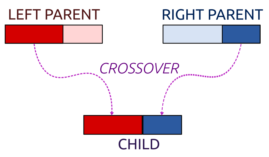
Figure 8.2: Crossover

crossover <- function(pop, pairs, K, p) {
    old_pop <- pop
    pop <- pop[pairs[,2]]
    for (j in 1:length(pop)) {
        wh <- sample(p-1, K, replace=TRUE)
        for (l in 1:K)
            pop[[j]][l,1:wh[l]] <-
                old_pop[[pairs[j,1]]][l,1:wh[l]]
    }
    pop
}

Mutation (occurring with a very small probability) substitutes some cluster centre with a random vector from the input dataset.

mutate <- function(pop, X, K) {
    for (j in 1:length(pop)) {
       if (runif(1) < 0.025) {
          szw <- sample(1:K, 1)
          pop[[j]][szw,] <- X[sample(nrow(X), length(szw)),]
       }
    }
    pop
}

We also need a function that checks if the new cluster centres aren’t too far away from the input points.

If it happens that we have empty clusters, our solution is degenerate and we must correct it.

All “bad” cluster centres will be substituted with randomly chosen points from \(\mathbf{X}\).

Moreover, we will recompute the cluster centres as the componentwise arithmetic mean of the closest points, just like in Lloyd’s algorithm, to speed up convergence.

recompute_mus <- function(pop, X, K) {
  for (j in 1:length(pop)) {
    # get nearest cluster centres for each point:
    memb <- get.knnx(pop[[j]], X, 1)$nn.index
    sz <- tabulate(memb, K) # number of points in each cluster
    # if there are empty clusters, fix them:
    szw <- which(sz==0)
    if (length(szw)>0) { # random points in X will be new cluster centres
        pop[[j]][szw,] <- X[sample(nrow(X), length(szw)),]
        memb <- FNN::get.knnx(pop[[j]], X, 1)$nn.index
        sz <- tabulate(memb, K)
    }
    # recompute cluster centres - componentwise average:
    pop[[j]][,] <- 0
    for (l in 1:nrow(X))
        pop[[j]][memb[l],] <- pop[[j]][memb[l],]+X[l,]
    pop[[j]] <- pop[[j]]/sz
  }
  pop
}

We are ready to build our genetic algorithm to solve the K-means clustering problem:

for (i in 1:niter) {
    pairs <- selection(cur_loss)
    pop <- crossover(pop, pairs, K, p)
    pop <- mutate(pop, X, K)
    pop <- recompute_mus(pop, X, K)
    # re-evaluate losses:
    cur_loss <- sapply(pop, get_loss, X)
    cur_best_loss <- min(cur_loss)
    # give feedback on what's going on:
    if (cur_best_loss < best_loss) {
        best_loss <- cur_best_loss
        best_mu <- pop[[which.min(cur_loss)]]
        cat(sprintf("%5d: f_best=%10.5f\n", i, best_loss))
    }
}

##     1: f_best=435638.52165
##     2: f_best=428808.89706
##     4: f_best=428438.45125
##     6: f_best=422277.99136
##     8: f_best=421889.46265

print(get_loss(best_mu, X))

## [1] 421889

print(get_loss(res_tried_very_hard, X))

## [1] 421889

It works! :)

8.3.1 Remarks

For any \(p\ge 1\), the search space type determines the problem class:

• \(\mathbb{D}\subseteq\mathbb{R}^p\) – continuous optimisation

  In particular:

  • \(\mathbb{D}=\mathbb{R}^p\) – continuous unconstrained

  • \(\mathbb{D}=[a_1,b_1]\times\dots\times[a_n,b_n]\) – continuous with box constraints

  • constrained with \(k\) linear inequality constraints

    \[ \left\{ \begin{array}{lll} a_{1,1} x_1 + \dots + a_{1,p} x_p &\le& b_1 \\ &\vdots&\\ a_{k,1} x_1 + \dots + a_{k,p} x_p &\le& b_k \\ \end{array} \right. \]

However, there are other possibilities as well:

• \(\mathbb{D}\subseteq\mathbb{Z}^p\) (\(\mathbb{Z}\) – the set of integers) – discrete optimisation

  In particular:

  • \(\mathbb{D}=\{0,1\}^p\) – 0–1 optimisation (hard!)

• \(\mathbb{D}\) is finite (but perhaps large, its objects can be enumerated) – combination optimisation

  For example:

  • \(\mathbb{D}=\) all possible routes between two points on a map.

These optimisation tasks tend to be much harder than the continuous ones.

Genetic algorithms might come in handy in such cases.

Specialised methods, customised to solve a specific problem (like Lloyd’s algorithm) will often outperform generic ones (like SGD, genetic algorithms) in terms of speed and reliability.

All in all, we prefer a suboptimal solution obtained by means of heuristics to no solution at all.

Problems that you could try solving with GAs include variable selection in multiple regression – finding the subset of features optimising the AIC (this is a hard problem to and forward selection was just a simple greed heuristic).

Other interesting algorithms:

• Hill Climbing (a simple variation of GD with no gradient use)
• Simulated annealing
• CMA-ES
• Tabu search
• Particle swarm optimisation (e.g, hydroPSO package)
• Artificial bee/ant colony optimisation
• Cuckoo Search
• Differential Evolution (e.g., DEoptim package)

8.3.2 Further Reading