C Vector Algebra in R

C.2.1 Creating Numeric Vectors

First let’s introduce a few ways with which we can create numeric vectors.

c(1, 2, 3)

## [1] 1 2 3

c(1, 2, 3, c(4, 5), c(6, c(7, 8)))

## [1] 1 2 3 4 5 6 7 8

x <- c(1, 2, 3) # doesn't print anything
print(x)

## [1] 1 2 3

(x <- c(1, 2, 3))

## [1] 1 2 3

mode(x)

## [1] "numeric"

class(x)

## [1] "numeric"

length(x)

## [1] 3

seq(1, 9, 2)

## [1] 1 3 5 7 9

seq(from=1, to=9, by=2)

## [1] 1 3 5 7 9

seq(0, 1, length.out=5)

## [1] 0.00 0.25 0.50 0.75 1.00

seq(0, 1, len=5)

## [1] 0.00 0.25 0.50 0.75 1.00

1:10     # from:to (inclusive)

##  [1]  1  2  3  4  5  6  7  8  9 10

-1:-10

##  [1]  -1  -2  -3  -4  -5  -6  -7  -8  -9 -10

rep(1, 5)

## [1] 1 1 1 1 1

rep(1:3, 4)

##  [1] 1 2 3 1 2 3 1 2 3 1 2 3

rep(1:3, c(2, 4, 3))

## [1] 1 1 2 2 2 2 3 3 3

rep(1:3, each=4)

##  [1] 1 1 1 1 2 2 2 2 3 3 3 3

C.2.1.4 Pseudo-Random Vectors

We can also generate vectors of pseudo-random values. For instance, the following generates 5 deviates from the uniform distribution (every number has the same probability) on the unit (i.e., \([0,1]\)) interval:

runif(5, 0, 1)

## [1] 0.56490 0.55881 0.44148 0.20764 0.66964

We call such numbers pseudo-random, because they are generated arithmetically. In fact, by setting the random number generator’s state (also called the seed), we can obtain reproducible results.

set.seed(123)
runif(5, 0, 1) # a,b,c,d,e

## [1] 0.28758 0.78831 0.40898 0.88302 0.94047

runif(5, 0, 1) # f,g,h,i,j

## [1] 0.045556 0.528105 0.892419 0.551435 0.456615

set.seed(123)
runif(5, 0, 1) # a,b,c,d,e again!

## [1] 0.28758 0.78831 0.40898 0.88302 0.94047

Note the difference between the uniform distribution on \([0,1]\) and the normal distribution with expected value of \(0\) and standard deviation of \(1\) (also called the standard normal distribution), see Figure C.1.

par(mfrow=c(1, 2)) # align plots in one row and two columns
hist(runif(10000, 0, 1), col="white", ylim=c(0, 2500)); box()
hist(rnorm(10000, 0, 1), col="white", ylim=c(0, 2500)); box()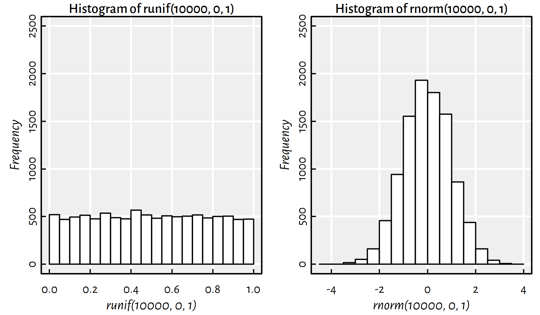

Figure C.1: Uniformly vs. normally distributed random variables

Another useful function samples a number of values from a given vector, either with or without replacement:

sample(1:10, 8, replace=TRUE) # with replacement

## [1]  3  3 10  2  6  5  4  6

sample(1:10, 8, replace=FALSE) # without replacement

## [1]  9  5  3  8  1  4  6 10

Note that if n is a single number, sample(n, ...) is equivalent to sample(1:n, ...). This is a dangerous behaviour than may lead to bugs in our code. Read more at ?sample.

C.2.2 Vector-Scalar Operations

Mathematically, we sometimes refer to a vector that is reduced to a single component as a scalar. We are used to denoting such objects with lowercase letters such as \(a, b, i, s, x\in\mathbb{R}\).

Remark.

Note that some programming languages distinguish between atomic numerical entities and length-one vectors, e.g., 7 vs. [7] in Python. This is not the case in R, where length(7) returns 1.

Vector-scalar arithmetic operations such as \(s\boldsymbol{x}\) (multiplication of a vector \(\boldsymbol{x}=(x_1,\dots, x_n)\) by a scalar \(s\)) result in a vector \(\boldsymbol{y}\) such that \(y_i=s x_i\), \(i=1,\dots,n\).

The same rule holds for, e.g., \(s+\boldsymbol{x}\), \(\boldsymbol{x}-s\), \(\boldsymbol{x}/s\).

0.5 * c(1, 10, 100)

## [1]  0.5  5.0 50.0

10 + 1:5

## [1] 11 12 13 14 15

seq(0, 10, by=2)/10

## [1] 0.0 0.2 0.4 0.6 0.8 1.0

By \(-\boldsymbol{x}\) we will mean \((-1)\boldsymbol{x}\):

-seq(0, 1, length.out=5)

## [1]  0.00 -0.25 -0.50 -0.75 -1.00

Note that in R the same rule applies for exponentiation:

(0:5)^2 # synonym: (1:5)**2

## [1]  0  1  4  9 16 25

2^(0:5)

## [1]  1  2  4  8 16 32

However, in mathematics, we are not used to writing \(2^{\boldsymbol{x}}\) or \(\boldsymbol{x}^2\).

C.2.3 Vector-Vector Operations

Let \(\boldsymbol{x}=(x_1,\dots,x_n)\) and \(\boldsymbol{y}=(y_1,\dots,y_n)\) be two vectors of identical lengths.

Arithmetic operations \(\boldsymbol{x}+\boldsymbol{y}\) and \(\boldsymbol{x}-\boldsymbol{y}\) are performed elementwise, i.e., they result in a vector \(\boldsymbol{z}\) such that \(z_i=x_i+y_i\) and \(z_i=x_i-y_i\), respectively, \(i=1,\dots,n\).

x <- c(1,  2,   3,    4)
y <- c(1, 10, 100, 1000)
x+y

## [1]    2   12  103 1004

x-y

## [1]    0   -8  -97 -996

Although in mathematics we are not used to using any special notation for elementwise multiplication, division and exponentiation, this is available in R.

x*y

## [1]    1   20  300 4000

x/y

## [1] 1.000 0.200 0.030 0.004

y^x

## [1] 1e+00 1e+02 1e+06 1e+12

Remark.

1e+12 is a number written in the scientific notation. It means “1 times 10 to the power of 12”, i.e., \(1\times 10^{12}\). Physicists love this notation, because they are used to dealing with very small (think sizes of quarks) and very large (think distances between galaxies) entities.

Moreover, in R the recycling rule is applied if we perform elementwise operations on vectors of different lengths – the shorter vector is recycled as many times as needed to match the length of the longer vector, just as if we were performing:

rep(1:3, length.out=12) # recycle 1,2,3 to get 12 values

##  [1] 1 2 3 1 2 3 1 2 3 1 2 3

Therefore:

1:6 * c(1)

## [1] 1 2 3 4 5 6

1:6 * c(1,10)

## [1]  1 20  3 40  5 60

1:6 * c(1,10,100)

## [1]   1  20 300   4  50 600

1:6 * c(1,10,100,1000)

## Warning in 1:6 * c(1, 10, 100, 1000): longer object length is not a
## multiple of shorter object length

## [1]    1   20  300 4000    5   60

Note that a warning is not an error – we still get a result that makes sense.

C.2.4 Aggregation Functions

R implements a couple of aggregation functions:

• sum(x) = \(\sum_{i=1}^n x_i=x_1+x_2+\dots+x_n\)
• prod(x) = \(\prod_{i=1}^n x_i=x_1 x_2 \dots x_n\)
• mean(x) = \(\frac{1}{n}\sum_{i=1}^n x_i\) – arithmetic mean
• var(x) = sum((x-mean(x))^2)/(length(x)-1) = \(\frac{1}{n-1} \sum_{i=1}^n \left(x_i - \frac{1}{n}\sum_{j=1}^n x_j \right)^2\) – variance
• sd(x) = sqrt(var(x)) – standard deviation

see also: min(), max(), median(), quantile().

Remark.

Remember that you can always access the R manual by typing ?functionname, e.g., ?quantile.

Remark.

Note that \(\sum_{i=1}^n x_i\) can also be written as \(\displaystyle\sum_{i=1}^n x_i\) or even \(\displaystyle\sum_{i=1,\dots,n} x_i\). These all mean the sum of \(x_i\) for \(i\) from \(1\) to \(n\), that is, the sum of \(x_1\), \(x_2\), …, \(x_n\), i.e., \(x_1+x_2+\dots+x_n\).

x <- runif(1000)
mean(x)

## [1] 0.49728

median(x)

## [1] 0.48995

min(x)

## [1] 0.00046535

max(x)

## [1] 0.9994

C.2.5 Special Functions

Furthermore, R supports numerous mathematical functions, e.g., sqrt(), abs(), round(), log(), exp(), cos(), sin(). All of them are vectorised – when applied on a vector of length \(n\), they yield a vector of length \(n\) in result.

For example, here is how we can compute the square roots of all the integers between 1 and 9:

sqrt(1:9)

## [1] 1.0000 1.4142 1.7321 2.0000 2.2361 2.4495 2.6458 2.8284 3.0000

Vectorisation is super-convenient when it comes to, for instance, plotting (see Figure C.2).

x <- seq(-2*pi, 6*pi, length.out=51)
plot(x, sin(x), type="l")
lines(x, cos(x), col="red") # add a curve to the current plot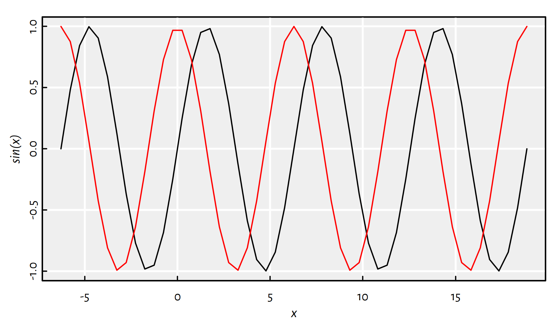

Figure C.2: An example plot of the sine and cosine functions

C.2.6 Norms and Distances

Norms are used to measure the size of an object. Mathematically, we will also be interested in the following norms:

• Euclidean norm: \[ \|\boldsymbol{x}\| = \|\boldsymbol{x}\|_2 = \sqrt{ \sum_{i=1}^n x_i^2 } \] this is nothing else than the length of the vector \(\boldsymbol{x}\)
• Manhattan (taxicab) norm: \[ \|\boldsymbol{x}\|_1 = \sum_{i=1}^n |x_i| \]
• Chebyshev (maximum) norm: \[ \|\boldsymbol{x}\|_\infty = \max_{i=1,\dots,n} |x_i| = \max\{ |x_1|, |x_2|, \dots, |x_n| \} \]

The above norms can be easily implemented by means of the building blocks introduced above. This is super easy:

z <- c(1, 2)
sqrt(sum(z^2)) # or norm(z, "2"); Euclidean

## [1] 2.2361

sum(abs(z))    # Manhattan

## [1] 3

max(abs(z))    # Chebyshev

## [1] 2

Also note that all the norms easily generate the corresponding distances (metrics) between two given points. In particular:

\[ \| \boldsymbol{x}-\boldsymbol{y} \| = \sqrt{ \sum_{i=1}^n \left(x_i-y_i\right)^2 } \]

gives the Euclidean distance (metric) between the two vectors.

u <- c(1, 0)
v <- c(1, 1)
sqrt(sum((u-v)^2))

## [1] 1

This is the “normal” distance that you learned at school.

C.2.7 Dot Product (*)

What is more, given two vectors of identical lengths, \(\boldsymbol{x}\) and \(\boldsymbol{y}\), we define their dot product (a.k.a. scalar or inner product) as:

\[ \boldsymbol{x}\cdot\boldsymbol{y} = \sum_{i=1}^n x_i y_i. \]

Let’s stress that this is not the same as the elementwise vector multiplication in R – the result is a single number.

u <- c(1, 0)
v <- c(1, 1)
sum(u*v)

## [1] 1

Remark.

(*) Note that the squared Euclidean norm of a vector is equal to the dot product of the vector and itself, \(\|\boldsymbol{x}\|^2 = \boldsymbol{x}\cdot\boldsymbol{x}\).

(*) Interestingly, a dot product has a nice geometrical interpretation: \[ \boldsymbol{x}\cdot\boldsymbol{y} = \|\boldsymbol{x}\| \|\boldsymbol{y}\| \cos\alpha \] where \(\alpha\) is the angle between the two vectors. In other words, it is the product of the lengths of the two vectors and the cosine of the angle between them. Note that we can get the cosine part by computing the dot product of the normalised vectors, i.e., such that their lengths are equal to 1.

For example, the two vectors u and v defined above can be depicted as in Figure C.3.

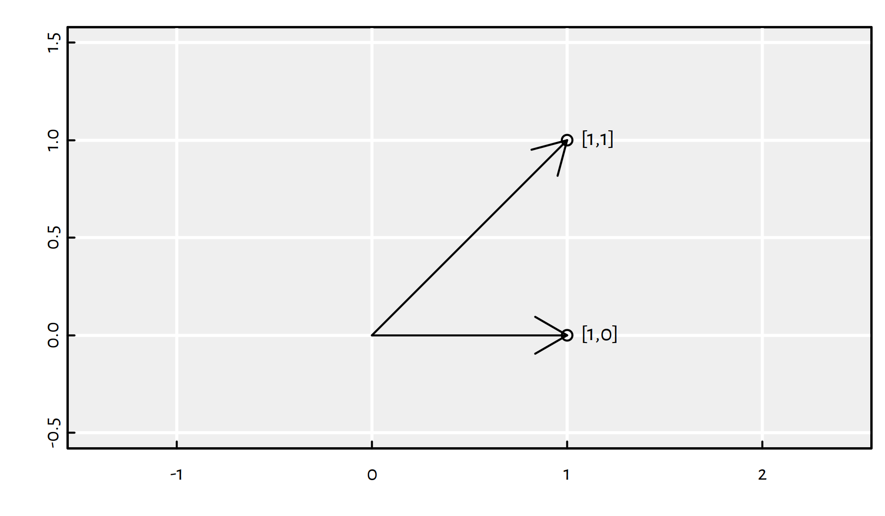
Figure C.3: Example vectors in 2D

We can compute the angle between them by calling:

(len_u <- sqrt(sum(u^2))) # length == Euclidean norm

## [1] 1

(len_v <- sqrt(sum(v^2)))

## [1] 1.4142

(cos_angle_uv <- (sum(u*v)/(len_u*len_v))) # cosine of the angle

## [1] 0.70711

acos(cos_angle_uv)*180/pi # angle in degs

## [1] 45

C.2.8 Missing and Other Special Values

R has a notion of a missing (not-available) value. It is very useful in data analysis, as we sometimes don’t have an information on an object’s feature. For instance, we might not know a patient’s age if he was admitted to the hospital unconscious.

x <- c(1, 2, NA, 4, 5)

Operations on missing values generally result in missing values – that makes a lot sense.

x + 11:15

## [1] 12 14 NA 18 20

mean(x)

## [1] NA

If we wish to compute a vector’s aggregate after all, we can get rid of the missing values by calling na.omit():

mean(na.omit(x)) # mean of non-missing values

## [1] 3

We can also make use of the na.rm parameter of the mean() function (however, not every aggregation function has it – always refer to documentation).

mean(x, na.rm=TRUE)

## [1] 3

Remark.

Note that in R, a dot has no special meaning. na.omit is as good of a function’s name or variable identifier as na_omit, naOmit, NAOMIT, naomit and NaOmit. Note that, however, R is a case-sensitive language – these are all different symbols. Read more in the Details section of ?make.names.

Moreover, some arithmetic operations can result in infinities (\(\pm \infty\)):

log(0)

## [1] -Inf

10^1000 # too large

## [1] Inf

Also, sometimes we’ll get a not-a-number, NaN. This is not a missing value, but a “invalid” result.

sqrt(-1)

## Warning in sqrt(-1): NaNs produced

## [1] NaN

log(-1)

## Warning in log(-1): NaNs produced

## [1] NaN

Inf-Inf

## [1] NaN

C.3.1 Creating Logical Vectors

In R there are 3 (!) logical values: TRUE, FALSE and geez, I don’t know, NA maybe?

c(TRUE, FALSE, TRUE, NA, FALSE, FALSE, TRUE)

## [1]  TRUE FALSE  TRUE    NA FALSE FALSE  TRUE

(x <- rep(c(TRUE, FALSE, NA), 2))

## [1]  TRUE FALSE    NA  TRUE FALSE    NA

mode(x)

## [1] "logical"

class(x)

## [1] "logical"

length(x)

## [1] 6

Remark.

By default, T is a synonym for TRUE and F for FALSE. This may be changed though so it’s better not to rely on these.

C.3.2 Logical Operations

Logical operators such as & (and) and | (or) are performed in the same manner as arithmetic ones, i.e.:

• they are elementwise operations and
• recycling rule is applied if necessary.

For example,

TRUE & TRUE

## [1] TRUE

TRUE & c(TRUE, FALSE)

## [1]  TRUE FALSE

c(FALSE, FALSE, TRUE, TRUE) | c(TRUE, FALSE, TRUE, FALSE)

## [1]  TRUE FALSE  TRUE  TRUE

The ! operator stands for logical elementwise negation:

!c(TRUE, FALSE)

## [1] FALSE  TRUE

Generally, operations on NAs yield NA unless other solution makes sense.

u <- c(TRUE, FALSE, NA)
v <- c(TRUE, TRUE, TRUE, FALSE, FALSE, FALSE, NA, NA, NA)
u & v # elementwise AND (conjunction)

## [1]  TRUE FALSE    NA FALSE FALSE FALSE    NA FALSE    NA

u | v # elementwise OR  (disjunction)

## [1]  TRUE  TRUE  TRUE  TRUE FALSE    NA  TRUE    NA    NA

!u    # elementwise NOT (negation)

## [1] FALSE  TRUE    NA

C.3.3 Comparison Operations

We can compare the corresponding elements of two numeric vectors and get a logical vector in result. Operators such as < (less than), <= (less than or equal), == (equal), != (not equal), > (greater than) and >= (greater than or equal) are again elementwise and use the recycling rule if necessary.

3 < 1:5 # c(3, 3, 3, 3, 3) < c(1, 2, 3, 4, 5)

## [1] FALSE FALSE FALSE  TRUE  TRUE

1:2 == 1:4 # c(1,2,1,2) == c(1,2,3,4)

## [1]  TRUE  TRUE FALSE FALSE

z <- c(0, 3, -1, 1, 0.5)
(z >= 0) & (z <= 1)

## [1]  TRUE FALSE FALSE  TRUE  TRUE

C.3.4 Aggregation Functions

Also note the following operations on logical vectors:

z <- 1:10
all(z >= 5) # are all values TRUE?

## [1] FALSE

any(z >= 5) # is there any value TRUE?

## [1] TRUE

Moreover:

sum(z >= 5) # how many TRUE values are there?

## [1] 6

mean(z >= 5) # what is the proportion of TRUE values?

## [1] 0.6

The behaviour of sum() and mean() is dictated by the fact that, when interpreted in numeric terms, TRUE is interpreted as numeric 1 and FALSE as 0.

as.numeric(c(FALSE, TRUE))

## [1] 0 1

Therefore in the example above we have:

z >= 5

##  [1] FALSE FALSE FALSE FALSE  TRUE  TRUE  TRUE  TRUE  TRUE  TRUE

as.numeric(z >= 5)

##  [1] 0 0 0 0 1 1 1 1 1 1

sum(as.numeric(z >= 5)) # the same as sum(z >= 5)

## [1] 6

Yes, there are 6 values equal to TRUE (or 6 ones after conversion), the sum of zeros and ones gives the number of ones.

C.4.1 Creating Character Vectors

Individual character strings can be created using double quotes or apostrophes. These are the elements of character vectors

(x <- "a string")

## [1] "a string"

mode(x)

## [1] "character"

class(x)

## [1] "character"

length(x)

## [1] 1

rep(c("aaa", 'bb', "c"), 2)

## [1] "aaa" "bb"  "c"   "aaa" "bb"  "c"

C.4.2 Concatenating Character Vectors

To join (concatenate) the corresponding elements of two or more character vectors, we call the paste() function:

paste(c("a", "b", "c"), c("1", "2", "3"))

## [1] "a 1" "b 2" "c 3"

paste(c("a", "b", "c"), c("1", "2", "3"), sep="")

## [1] "a1" "b2" "c3"

Also note:

paste(c("a", "b", "c"), 1:3) # the same as as.character(1:3)

## [1] "a 1" "b 2" "c 3"

paste(c("a", "b", "c"), 1:6) # recycling

## [1] "a 1" "b 2" "c 3" "a 4" "b 5" "c 6"

paste(c("a", "b", "c"), 1:6, c("!", "?"))

## [1] "a 1 !" "b 2 ?" "c 3 !" "a 4 ?" "b 5 !" "c 6 ?"

C.4.3 Collapsing Character Vectors

We can also collapse a sequence of strings to a single string:

paste(c("a", "b", "c", "d"), collapse="")

## [1] "abcd"

paste(c("a", "b", "c", "d"), collapse=",")

## [1] "a,b,c,d"

C.5.1 Subsetting with Positive Indices

In order to extract subsets (parts) of vectors, we use the square brackets:

(x <- seq(10, 100, 10))

##  [1]  10  20  30  40  50  60  70  80  90 100

x[1]         # the first element

## [1] 10

x[length(x)] # the last element

## [1] 100

More than one element at a time can also be extracted:

x[1:3] # the first three

## [1] 10 20 30

x[c(1, length(x))] # the first and the last

## [1]  10 100

For example, the order() function returns the indices of the smallest, 2nd smallest, 3rd smallest, …, the largest element in a given vector. We will use this function when implementing our first classifier.

y <- c(50, 30, 10, 20, 40)
(o <- order(y))

## [1] 3 4 2 5 1

Hence, we see that the smallest element in y is at index 3 and the largest at index 1:

y[o[1]]

## [1] 10

y[o[length(y)]]

## [1] 50

Therefore, to get a sorted version of y, we call:

y[o] # see also sort(y)

## [1] 10 20 30 40 50

We can also obtain the 3 largest elements by calling:

y[order(y, decreasing=TRUE)[1:3]]

## [1] 50 40 30

C.5.2 Subsetting with Negative Indices

Subsetting with a vector of negative indices, excludes the elements at given positions:

x[-1] # all but the first

## [1]  20  30  40  50  60  70  80  90 100

x[-(1:3)]

## [1]  40  50  60  70  80  90 100

x[-c(1:3, 5, 8)]

## [1]  40  60  70  90 100

C.5.3 Subsetting with Logical Vectors

We may also subset a vector \(\boldsymbol{x}\) of length \(n\) with a logical vector \(\boldsymbol{l}\) also of length \(n\). The \(i\)-th element, \(x_i\), will be extracted if and only if the corresponding \(l_i\) is true.

x[c(TRUE, FALSE, FALSE, FALSE, TRUE, FALSE, TRUE, TRUE, FALSE)]

## [1]  10  50  70  80 100

This gets along nicely with comparison operators that yield logical vectors on output.

x>50

##  [1] FALSE FALSE FALSE FALSE FALSE  TRUE  TRUE  TRUE  TRUE  TRUE

x[x>50] # select elements in x that are greater than 50

## [1]  60  70  80  90 100

x[x<30 | x>70]

## [1]  10  20  80  90 100

x[x<max(x)] # getting rid of the greatest element

## [1] 10 20 30 40 50 60 70 80 90

x[x > min(x) & x < max(x)] # return all but the smallest and greatest one

## [1] 20 30 40 50 60 70 80 90

Of course, e.g., x[x<max(x)] returns a new, independent object. In order to remove the greatest element in x permanently, we can write x <- x[x<max(x)].

C.5.4 Replacing Elements

Note that the three above vector indexing schemes (positive, negative, logical indices) allow for replacing specific elements with new values.

x[-1] <- 10000
x

##  [1]    10 10000 10000 10000 10000 10000 10000 10000 10000 10000

x[-(1:7)] <- c(1, 2, 3)
x

##  [1]    10 10000 10000 10000 10000 10000 10000     1     2     3

C.5.5 Other Functions

head() and tail() return, respectively, a few (6 by default) first and last elements of a vector.

head(x) # head(x, 6)

## [1]    10 10000 10000 10000 10000 10000

tail(x, 3)

## [1] 1 2 3

Sometimes the which() function can come in handy. For a given logical vector, it returns all the indices where TRUE elements are stored.

which(c(TRUE, FALSE, TRUE, TRUE, FALSE, FALSE, TRUE))

## [1] 1 3 4 7

print(y) # recall

## [1] 50 30 10 20 40

which(y>30)

## [1] 1 5

Note that y[y>70] gives the same result as y[which(y>70)] but is faster (because it involves less operations).

which.min() and which.max() return the index of the smallest and the largest element, respectively:

which.min(y) # where is the minimum?

## [1] 3

which.max(y)

## [1] 1

y[which.min(y)] # min(y)

## [1] 10

is.na() indicates which elements are missing values (NAs):

z <- c(1, 2, NA, 4, NA, 6)
is.na(z)

## [1] FALSE FALSE  TRUE FALSE  TRUE FALSE

Therefore, to remove them from z permanently, we can write (compare na.omit(), see also is.finite()):

(z <- z[!is.na(z)])

## [1] 1 2 4 6

C.6.1 Creating Named Vectors

Vectors in R can be named – each element can be assigned a string label.

x <- c(20, 40, 99, 30, 10)
names(x) <- c("a", "b", "c", "d", "e")
x # a named vector

##  a  b  c  d  e 
## 20 40 99 30 10

Other ways to create named vectors include:

c(a=1, b=2, c=3)

## a b c 
## 1 2 3

structure(1:3, names=c("a", "b", "c"))

## a b c 
## 1 2 3

For instance, the summary() function returns a named vector:

summary(x) # NAMED vector, we don't want this here yet

##    Min. 1st Qu.  Median    Mean 3rd Qu.    Max. 
##    10.0    20.0    30.0    39.8    40.0    99.0

This gives the minimum, 1st quartile (25%-quantile), Median (50%-quantile), aritmetic mean, 3rd quartile (75%-quantile) and maximum.

Note that x is still a numeric vector, we can perform various operations on it as usual:

sum(x)

## [1] 199

x[x>3]

##  a  b  c  d  e 
## 20 40 99 30 10

Names can be dropped by calling:

unname(x)

## [1] 20 40 99 30 10

as.numeric(x) # we need to know the type of x though

## [1] 20 40 99 30 10

C.6.2 Subsetting Named Vectors with Character String Indices

It turns out that extracting elements from a named vector can also be performed by means of a vector of character string indices:

x[c("a", "d", "b")]

##  a  d  b 
## 20 30 40

summary(x)[c("Median", "Mean")]

## Median   Mean 
##   30.0   39.8

C.7.1 Creating Factors

For example, the following character vector:

(col <- sample(c("blue", "red", "green"), replace=TRUE, 10))

##  [1] "green" "green" "green" "red"   "green" "red"   "red"   "red"  
##  [9] "green" "blue"

can be converted to a factor by calling:

(fcol <- factor(col))

##  [1] green green green red   green red   red   red   green blue 
## Levels: blue green red

Note how different is the way factors are printed out on the console.

C.7.2 Levels

We can easily obtain the list unique labels:

levels(fcol)

## [1] "blue"  "green" "red"

Those can be re-encoded by calling:

levels(fcol) <- c("b", "g", "r")
fcol

##  [1] g g g r g r r r g b
## Levels: b g r

To create a contingency table (in the form of a named numeric vector, giving how many values are at each factor level), we call:

table(fcol)

## fcol
## b g r 
## 1 5 4

C.7.3 Internal Representation (*)

Factors have a look-and-feel of character vectors, however, internally they are represented as integer sequences.

class(fcol)

## [1] "factor"

mode(fcol)

## [1] "numeric"

as.numeric(fcol)

##  [1] 2 2 2 3 2 3 3 3 2 1

These are always integers from 1 to M inclusive, where M is the number of levels. Their meaning is given by the levels() function: in the example above, the meaning of the codes 1, 2, 3 is, respectively, b, g, r.

If we wished to generate a factor with a specific order of labels, we could call:

factor(col, levels=c("red", "green", "blue"))

##  [1] green green green red   green red   red   red   green blue 
## Levels: red green blue

We can also assign different labels upon creation of a factor:

factor(col, levels=c("red", "green", "blue"), labels=c("r", "g", "b"))

##  [1] g g g r g r r r g b
## Levels: r g b

Knowing how factors are represented is important when we deal with factors that are built around data that look like numeric. This is because their conversion to numeric gives the internal codes, not the actual values:

(f <- factor(c(1, 3, 0, 1, 4, 0, 0, 1, 4)))

## [1] 1 3 0 1 4 0 0 1 4
## Levels: 0 1 3 4

as.numeric(f) # not necessarily what we want here

## [1] 2 3 1 2 4 1 1 2 4

as.numeric(as.character(f)) # much better

## [1] 1 3 0 1 4 0 0 1 4

Moreover, that idea is labour-saving in contexts such as plotting of data that are grouped into different classes. For instance, here is a scatter plot for the Sepal.Length and Petal.Width variables in the iris dataset (which is an object of type data.frame, see below). Flowers are of different Species, and we wish to indicate which point belongs to which class:

which_preview <- c(1, 11, 51, 69, 101) # indexes we show below
iris$Sepal.Length[which_preview]

## [1] 5.1 5.4 7.0 6.2 6.3

iris$Petal.Width[which_preview]

## [1] 0.2 0.2 1.4 1.5 2.5

iris$Species[which_preview]

## [1] setosa     setosa     versicolor versicolor virginica 
## Levels: setosa versicolor virginica

as.numeric(iris$Species)[which_preview]

## [1] 1 1 2 2 3

plot(iris$Sepal.Length, # x (it's a vector)
     iris$Petal.Width,  # y (it's a vector)
     col=as.numeric(iris$Species), # colours
     pch=as.numeric(iris$Species)
)

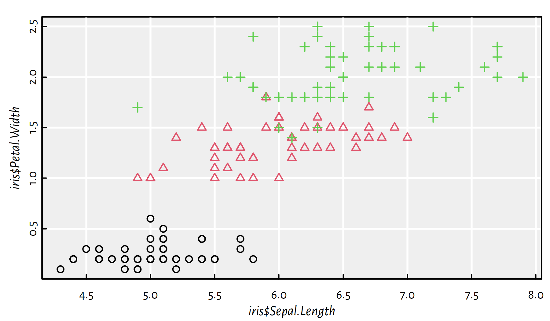
Figure C.4: as.numeric() on factors can be used to create different plotting styles

The above (see Figure C.4) was possible because the Species column is a factor object with:

levels(iris$Species)

## [1] "setosa"     "versicolor" "virginica"

and the meaning of pch of 1, 2, 3, … is “circle”, “triangle”, “plus”, …, respectively. What’s more, there’s a default palette that maps consecutive integers to different colours:

palette()

## [1] "black"   "#DF536B" "#61D04F" "#2297E6" "#28E2E5" "#CD0BBC"
## [7] "#F5C710" "gray62"

Hence, black circles mark irises from the 1st class, i.e., “setosa”.

C.8.1 Creating Lists

Most commonly, we create a generalised vector by calling the list() function.

(l <- list(1:5, letters, runif(3)))

## [[1]]
## [1] 1 2 3 4 5
## 
## [[2]]
##  [1] "a" "b" "c" "d" "e" "f" "g" "h" "i" "j" "k" "l" "m" "n" "o" "p" "q"
## [18] "r" "s" "t" "u" "v" "w" "x" "y" "z"
## 
## [[3]]
## [1] 0.95683 0.45333 0.67757

mode(l)

## [1] "list"

class(l)

## [1] "list"

length(l)

## [1] 3

There’s a more compact way to print a list on the console:

str(l)

## List of 3
##  $ : int [1:5] 1 2 3 4 5
##  $ : chr [1:26] "a" "b" "c" "d" ...
##  $ : num [1:3] 0.957 0.453 0.678

We can also convert an atomic vector to a list by calling:

as.list(1:3)

## [[1]]
## [1] 1
## 
## [[2]]
## [1] 2
## 
## [[3]]
## [1] 3

C.8.2 Named Lists

List, like other vectors, may be assigned a names attribute.

names(l) <- c("a", "b", "c")
l

## $a
## [1] 1 2 3 4 5
## 
## $b
##  [1] "a" "b" "c" "d" "e" "f" "g" "h" "i" "j" "k" "l" "m" "n" "o" "p" "q"
## [18] "r" "s" "t" "u" "v" "w" "x" "y" "z"
## 
## $c
## [1] 0.95683 0.45333 0.67757

C.8.3 Subsetting and Extracting From Lists

Applying a square brackets operator creates a sub-list, which is of type list as well.

l[-1]

## $b
##  [1] "a" "b" "c" "d" "e" "f" "g" "h" "i" "j" "k" "l" "m" "n" "o" "p" "q"
## [18] "r" "s" "t" "u" "v" "w" "x" "y" "z"
## 
## $c
## [1] 0.95683 0.45333 0.67757

l[c("a", "c")]

## $a
## [1] 1 2 3 4 5
## 
## $c
## [1] 0.95683 0.45333 0.67757

l[1]

## $a
## [1] 1 2 3 4 5

Note in the 3rd case we deal with a list of length one, not a numeric vector.

To extract (dig into) a particular (single) element, we use double square brackets:

l[[1]]

## [1] 1 2 3 4 5

l[["c"]]

## [1] 0.95683 0.45333 0.67757

The latter can equivalently be written as:

l$c

## [1] 0.95683 0.45333 0.67757

C.8.4 Common Operations

Lists, because of their generality (they can store any kind of object), have few dedicated operations. In particular, it neither makes sense to add, multiply, … two lists together nor to aggregate them.

However, if we wish to run some operation on each element, we can call list-apply:

(k <- list(x=runif(5), y=runif(6), z=runif(3))) # a named list

## $x
## [1] 0.57263 0.10292 0.89982 0.24609 0.04206
## 
## $y
## [1] 0.32792 0.95450 0.88954 0.69280 0.64051 0.99427
## 
## $z
## [1] 0.65571 0.70853 0.54407

lapply(k, mean)

## $x
## [1] 0.37271
## 
## $y
## [1] 0.74992
## 
## $z
## [1] 0.6361

The above computes the mean of each of the three numeric vectors stored inside list k. Moreover:

lapply(k, range)

## $x
## [1] 0.04206 0.89982
## 
## $y
## [1] 0.32792 0.99427
## 
## $z
## [1] 0.54407 0.70853

The built-in function range(x) returns c(min(x), max(x)).

unlist() tries (it might not always be possible) to unwind a list to a simpler, atomic form:

unlist(lapply(k, mean))

##       x       y       z 
## 0.37271 0.74992 0.63610

Moreover, split(x, f) classifies elements in a vector x into subgroups defined by a factor (or an object coercible to) of the same length.

x <- c(  1,   2,   3,   4,   5,   6,   7,   8,   9,  10)
f <- c("a", "b", "a", "a", "c", "b", "b", "a", "a", "b")
split(x, f)

## $a
## [1] 1 3 4 8 9
## 
## $b
## [1]  2  6  7 10
## 
## $c
## [1] 5

This is very useful when combined with lapply() and unlist(). For instance, here are the mean sepal lengths for each of the three flower species in the famous iris dataset.

unlist(lapply(split(iris$Sepal.Length, iris$Species), mean))

##     setosa versicolor  virginica 
##      5.006      5.936      6.588

By the way, if we take a look at the documentation of ?lapply, we will note that that this function is defined as lapply(X, FUN, ...). Here ... denotes the optional arguments that will be passed to FUN.

In other words, lapply(X, FUN, ...) returns a list Y of length length(X) such that Y[[i]] <- FUN(X[[i]], ...) for each i. For example, mean() has an additional argument na.rm that aims to remove missing values from the input vector. Compare the following:

t <- list(1:10, c(1, 2, NA, 4, 5))
unlist(lapply(t, mean))

## [1] 5.5  NA

unlist(lapply(t, mean, na.rm=TRUE))

## [1] 5.5 3.0

Of course, we can always pass a custom (self-made) function object as well:

min_mean_max <- function(x) {
    # the last expression evaluated in the function's body
    # gives its return value:
    c(min(x), mean(x), max(x))
}
lapply(k, min_mean_max)

## $x
## [1] 0.04206 0.37271 0.89982
## 
## $y
## [1] 0.32792 0.74992 0.99427
## 
## $z
## [1] 0.54407 0.63610 0.70853

or, more concisely (we can skip the curly braces here – they are normally used to group many expressions into one; also, if we don’t plan to re-use the function again, there’s no need to give it a name):

lapply(k, function(x) c(min(x), mean(x), max(x)))

## $x
## [1] 0.04206 0.37271 0.89982
## 
## $y
## [1] 0.32792 0.74992 0.99427
## 
## $z
## [1] 0.54407 0.63610 0.70853