7 Clustering

7.1.1 Introduction

In unsupervised learning (learning without a teacher), the input data points \(\mathbf{x}_{1,\cdot},\dots,\mathbf{x}_{n,\cdot}\) are not assigned any reference labels (compare Figure 7.1).

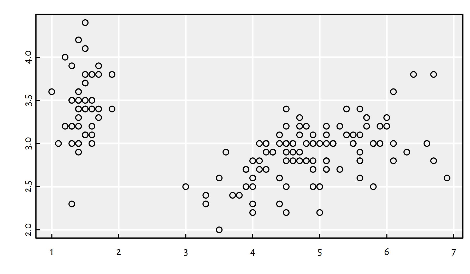
Figure 7.1: Unsupervised learning: “But what it is exactly that I have to do here?”

Our aim now is to discover the underlying structure in the data, whatever that means.

7.1.2 Main Types of Unsupervised Learning Problems

It turns out, however, that certain classes of unsupervised learning problems are not only intellectually stimulating, but practically useful at the same time.

In particular, in dimensionality reduction we seek a meaningful projection of a high dimensional space (think: many variables/columns).

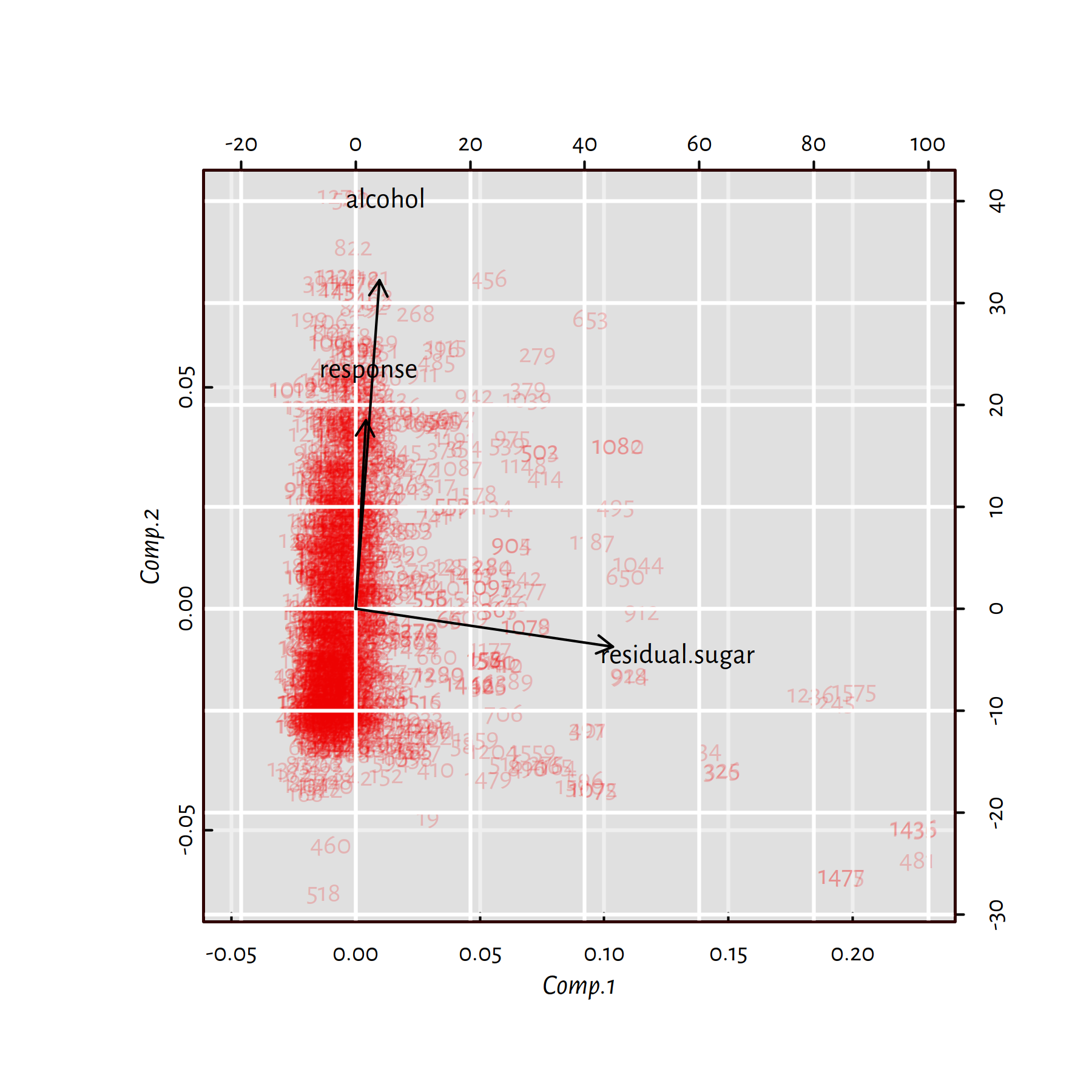
Figure 7.2: Principal component analysis (a dimensionality reduction technique) applied on three features of red wines

For instance, Figure 7.2 reveals that the “alcohol”, “response” and “residual.sugar” dimensions of the Wine Quality dataset that we have studied earlier on can actually be nicely depicted (with no much loss of information) on a two-dimensional plot. It turns out that the wine experts’ opinion on a wine’s quality is highly correlated with the amount of… alcohol in a bottle. On the other hand, sugar is orthogonal (unrelated) to these two.

Amongst example dimensionality reduction methods we find:

• Multidimensional scaling (MDS)
• Principal component analysis (PCA)
• Kernel PCA
• t-SNE
• Autoencoders (deep learning)

See, for example, (Hastie et al. 2017) for more details.

Furthermore, in anomaly detection, our task is to identify rare, suspicious, ab-normal or out-standing items. For example, these can be cars on walkways in a park’s security camera footage.

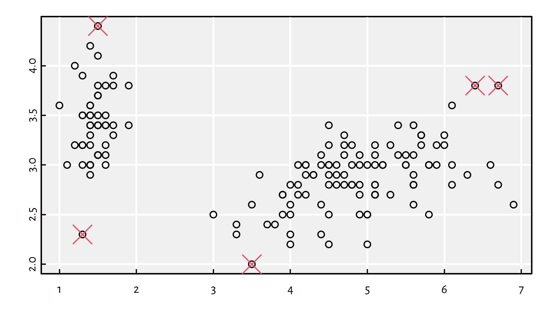
(#fig:anomaly_detection) Outliers can be thought of anomalies of some sort

Finally, the aim of clustering is to automatically discover some naturally occurring subgroups in the data set, compare Figure 7.3. For example, these may be customers having different shopping patterns (such as “young parents”, “students”, “boomers”).

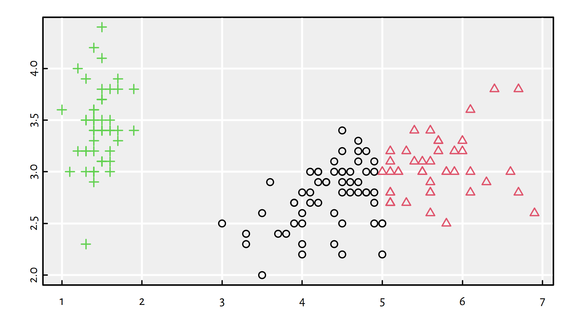
Figure 7.3: NEWS FLASH! SCIENTISTS SHOWED (by writing about it) THAT SOME VERY IMPORTANT THING (Iris dataset) COMES IN THREE DIFFERENT FLAVOURS (by applying the 3-means clustering algorithm)!

7.1.3 Definitions

Formally, given \(K\ge 2\), clustering aims is to find a special kind of a \(K\)-partition of the input data set \(\mathbf{X}\).

Definition.

We say that \(\mathcal{C}=\{C_1,\dots,C_K\}\) is a \(K\)-partition of \(\mathbf{X}\) of size \(n\), whenever:

• \(C_k\neq\emptyset\) for all \(k\) (each set is nonempty),
• \(C_k\cap C_l=\emptyset\) for all \(k\neq l\) (sets are pairwise disjoint),
• \(\bigcup_{k=1}^K C_k=\mathbf{X}\) (no point is neglected).

This can also be thought of as assigning each point a unique label \(\{1,\dots,K\}\) (think: colouring of the points, where each number has a colour). We will consider the point \(\mathbf{x}_{i,\cdot}\) as labelled \(j\) if and only if it belongs to cluster \(C_j\), i.e., \(\mathbf{x}_{i,\cdot}\in C_j\).

Example applications of clustering:

• taxonomisation: e.g., partition the consumers to more “uniform” groups to better understand who they are and what do they need,
• image processing: e.g., object detection, like tumour tissues on medical images,
• complex networks analysis: e.g., detecting communities in friendship, retweets and other networks,
• fine-tuning supervised learning algorithms: e.g., recommender systems indicating content that was rated highly by users from the same group or learning multiple manifolds in a dimension reduction task.

The number of possible \(K\)-partitions of a set with \(n\) elements is given by the Stirling number of the second kind:

\[ \left\{{n \atop K}\right\}={\frac {1}{K!}}\sum _{{j=0}}^{{K}}(-1)^{{K-j}}{\binom {K}{j}}j^{n}; \]

e.g., already \(\left\{{n \atop 2}\right\}=2^{n-1}-1\) and \(\left\{{n \atop 3}\right\}=O(3^n)\) – that is a lot. Certainly, we are not just interested in “any” partition – some of them will be more meaningful or valuable than others. However, even one of the most famous ML textbooks provides us with only a vague hint of what we might be looking for:

“Definition”.

Clustering concerns “segmenting a collection of objects into subsets so that those within each cluster are more closely related to one another than objects assigned to different clusters” (Hastie et al. 2017).

It is not uncommon to equate the general definition of data clustering problems with… the particular outputs yield by specific clustering algorithms. It some sense, that sounds fair. From this perspective, we might be interested in identifying the two main types of clustering algorithms:

• parametric (model-based):
  • find clusters of specific shapes or following specific multidimensional probability distributions,
  • e.g., \(K\)-means, expectation-maximisation for Gaussian mixtures (EM), average linkage agglomerative clustering;
• nonparametric (model-free):
  • identify high-density or well-separable regions, perhaps in the presence of noise points,
  • e.g., single linkage agglomerative clustering, Genie, (H)DBSCAN, BIRCH.

In this chapter we’ll take a look at two classical approaches to clustering:

• K-means clustering that looks for a specific number of clusters,
• (agglomerative) hierarchical clustering that outputs a whole hierarchy of nested data partitions.

7.2.1 Example in R

Let’s begin our clustering adventure by applying the \(K\)-means clustering method to find \(K=3\) groups in the famous Fisher’s iris data set (variables Sepal.Width and Petal.Length variables only):

X <- as.matrix(iris[,c(3,2)])
# never forget to set nstart>>1!
km <- kmeans(X, centers=3, nstart=10)
km$cluster # labels assigned to each of 150 points:

##  [1] 1 1 1 1 1 1 1 1 1 1 1 1 1 1 1 1 1 1 1 1 1 1 1 1 1 1 1 1 1 1 1 1 1 1
## [35] 1 1 1 1 1 1 1 1 1 1 1 1 1 1 1 1 3 3 3 3 3 3 3 3 3 3 3 3 3 3 3 3 3 3
## [69] 3 3 3 3 3 3 3 3 3 2 3 3 3 3 3 2 3 3 3 3 3 3 3 3 3 3 3 3 3 3 3
##  [ reached getOption("max.print") -- omitted 51 entries ]

Remark.

Later we’ll see that nstart is responsible for random restarting the (local) optimisation procedure, just as we did in the previous chapter.

Let’s draw a scatter plot that depicts the detected clusters:

plot(X, col=km$cluster)

Figure 7.4: 3-means clustering on a projection of the Iris dataset

The colours in Figure 7.4 indicate the detected clusters. The left group is clearly well-separated from the other two.

What can we do with this information? Well, if we were experts on plants (in the 1930s), that’d definitely be something ground-breaking. Figure 7.5 is a version of the aforementioned scatter plot now with the true iris species added.

plot(X, col=km$cluster, pch=as.numeric(iris$Species))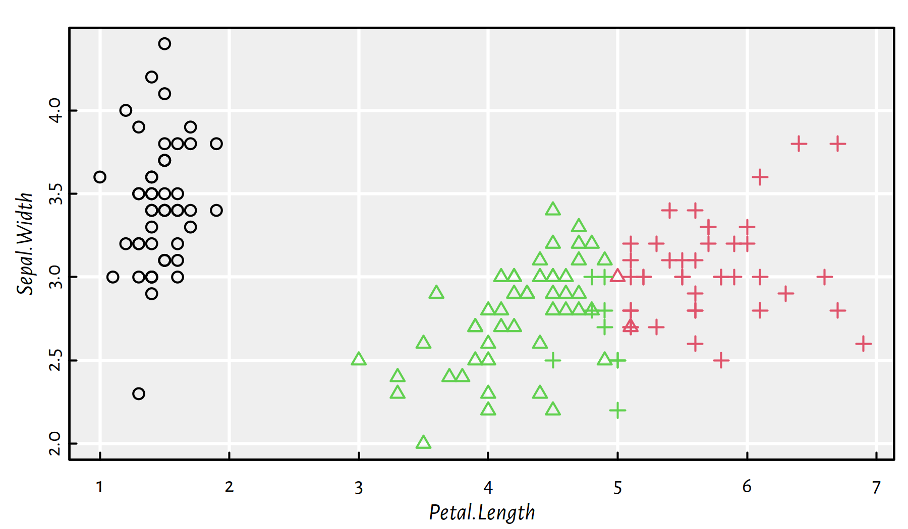

Figure 7.5: 3-means clustering (colours) vs true Iris species (shapes)

Here is a contingency table for detected clusters vs. true iris species:

(C <- table(km$cluster, iris$Species))

##    
##     setosa versicolor virginica
##   1     50          0         0
##   2      0          2        41
##   3      0         48         9

It turns out that the discovered partition matches the original iris species very well. We have just made a “discovery” in the field of botany (actually some research fields classify their objects of study into families, genres etc. by means of such tools).

Were the actual Iris species what we had hoped to match? Was that our aim? Well, surely we have had begun our journey with “clear minds” (yet with hungry eyes). Note that the true class labels were not used during the clustering procedure – we’re dealing with an unsupervised learning problem here. The result turned useful, it’s a win.

Remark.

(*) There are several indices that assess the similarity of two partitions, for example the Adjusted Rand Index (ARI) the Normalised Mutual Information Score (NMI) or set matching-based measures, see, e.g., (Hubert & Arabie 1985), (Rezaei & Fränti 2016).

7.2.2 Problem Statement

The aim of \(K\)-means clustering is to find \(K\) “good” cluster centres \(\boldsymbol\mu_{1,\cdot}, \dots, \boldsymbol\mu_{K,\cdot}\).

Then, a point \(\mathbf{x}_{i,\cdot}\) will be assigned to the cluster represented by the closest centre. Here, by closest we mean the squared Euclidean distance.

More formally, assuming all the points are in a \(p\)-dimensional space, \(\mathbb{R}^p\), we define the distance between the \(i\)-th point and the \(k\)-th centre as:

\[ d(\mathbf{x}_{i,\cdot}, \boldsymbol\mu_{k,\cdot}) = \| \mathbf{x}_{i,\cdot} - \boldsymbol\mu_{k,\cdot} \|^2 = \sum_{j=1}^p \left(x_{i,j}-\mu_{k,j}\right)^2 \]

Then the \(i\)-th point’s cluster is determined by:

\[ \mathrm{C}(i) = \mathrm{arg}\min_{k=1,\dots,K} d(\mathbf{x}_{i,\cdot}, \boldsymbol\mu_{k,\cdot}), \]

where, as usual, \(\mathrm{arg}\min\) (argument minimum) is the index \(k\) that minimises the given expression.

In the previous example, the three identified cluster centres in \(\mathbb{R}^2\) are given by (see Figure 7.6 for illustration):

km$centers

##   Petal.Length Sepal.Width
## 1       1.4620      3.4280
## 2       5.6721      3.0326
## 3       4.3281      2.7509

plot(X, col=km$cluster, asp=1) # asp=1 gives the same scale on both axes
points(km$centers, cex=2, col=4, pch=16)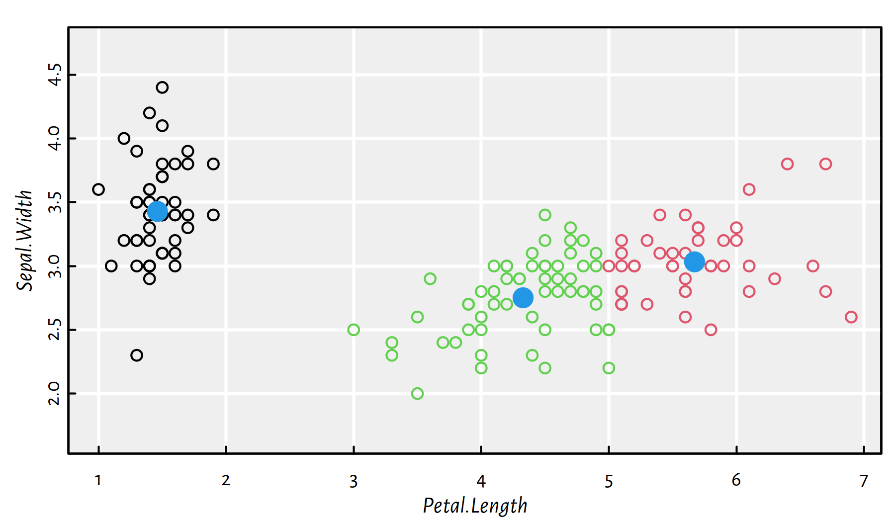

Figure 7.6: Cluster centres (blue dots) identified by the 3-means algorithm

Figure 7.7 depicts the partition of the whole \(\mathbb{R}^2\) space into clusters based on the closeness to the three cluster centres.

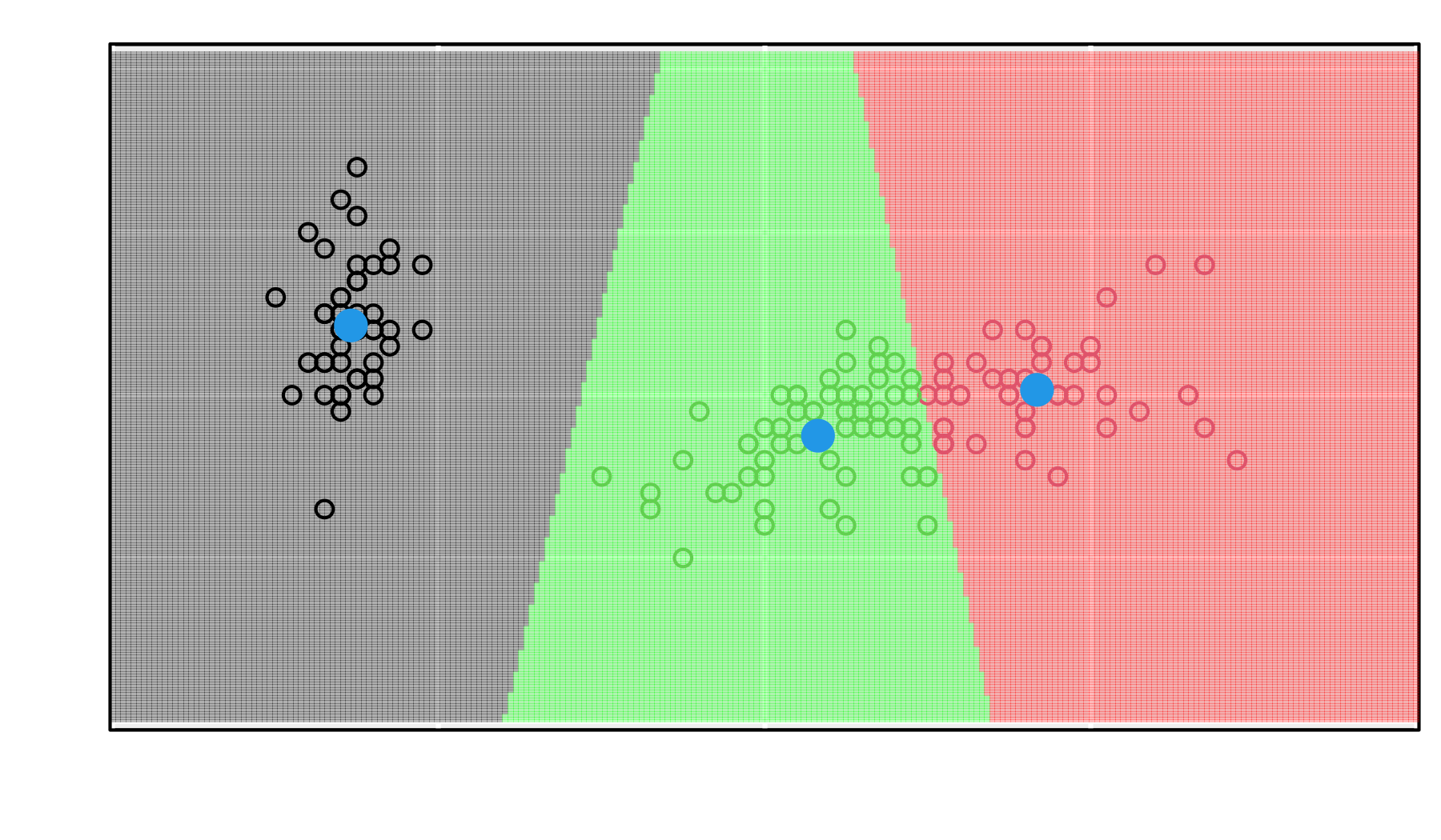
Figure 7.7: The division of the whole space into three sets based on the proximity to cluster centres (a so-called Voronoi diagram)

To compute the distances between all the points and the cluster centres, we may call pdist::pdist():

library("pdist")
D <- as.matrix(pdist(X, km$centers))^2
head(D)

##          [,1]   [,2]   [,3]
## [1,] 0.009028 18.469 9.1348
## [2,] 0.187028 18.252 8.6357
## [3,] 0.078228 19.143 9.3709
## [4,] 0.109028 17.411 8.1199
## [5,] 0.033428 18.573 9.2946
## [6,] 0.279428 16.530 8.2272

where D[i,k] gives the squared Euclidean distance between \(\mathbf{x}_{i,\cdot}\) and \(\boldsymbol\mu_{k,\cdot}\).

The cluster memberships the (\(\mathrm{arg}\min\)s) can now be determined by:

(idx <- apply(D, 1, which.min)) # for every row of D...

##  [1] 1 1 1 1 1 1 1 1 1 1 1 1 1 1 1 1 1 1 1 1 1 1 1 1 1 1 1 1 1 1 1 1 1 1
## [35] 1 1 1 1 1 1 1 1 1 1 1 1 1 1 1 1 3 3 3 3 3 3 3 3 3 3 3 3 3 3 3 3 3 3
## [69] 3 3 3 3 3 3 3 3 3 2 3 3 3 3 3 2 3 3 3 3 3 3 3 3 3 3 3 3 3 3 3
##  [ reached getOption("max.print") -- omitted 51 entries ]

all(km$cluster == idx) # sanity check

## [1] TRUE

7.2.3 Algorithms for the K-means Problem

All good, but how do we find “good” cluster centres? Good, better, best… yet again we are in a need for a goodness-of-fit metric. In the \(K\)-means clustering, we determine \(\boldsymbol\mu_{1,\cdot}, \dots, \boldsymbol\mu_{K,\cdot}\) that minimise the total within-cluster distances (distances from each point to each own cluster centre):

\[ \min_{\boldsymbol\mu_{1,\cdot}, \dots, \boldsymbol\mu_{K,\cdot} \in \mathbb{R}^p} \sum_{i=1}^n d(\mathbf{x}_{i,\cdot}, \boldsymbol\mu_{C(i),\cdot}), \]

Note that the \(\boldsymbol\mu\)s are also “hidden” inside the point-to-cluster belongingness mapping, \(\mathrm{C}\). Expanding the above yields:

\[ \min_{\boldsymbol\mu_{1,\cdot}, \dots, \boldsymbol\mu_{K,\cdot} \in \mathbb{R}^p} \sum_{i=1}^n \left( \min_{k=1,\dots,K} \sum_{j=1}^p \left(x_{i,j}-\mu_{k,j}\right)^2 \right). \]

Unfortunately, the \(\min\) operator in the objective function makes this optimisation problem not tractable with the methods discussed in the previous chapter.

The above problem is hard to solve (* more precisely, it is an NP-hard problem). Therefore, in practice we use various heuristics to solve it. The kmeans() function itself implements 3 of them: the Hartigan-Wong, Lloyd (a.k.a. Lloyd-Forgy) and MacQueen algorithms.

Remark.

(*) Technically, there is no such thing as “the K-means algorithm” – all the aforementioned methods are particular heuristic approaches to solving the K-means clustering problem formalised as the above optimisation task. By setting nstart = 10 above, we ask the (Hartigan-Wong, which is the default one in kmeans()) algorithm to find 10 solution candidates obtained by considering different random initial clusterings and choose the best one (with respect to the sum of within-cluster distances) amongst them. This does not guarantee finding the optimal solution, especially for very unbalanced datasets, but increases the likelihood of such.

Remark.

The squared Euclidean distance was of course chosen to make computations easier. It turns out that for any given subset of input points \(\mathbf{x}_{i_1,\cdot},\dots,\mathbf{x}_{i_m,\cdot}\), the point \(\boldsymbol\mu_{k,\cdot}\) that minimises the total distances to all of them, i.e.,

\[ \min_{\boldsymbol\mu_{k,\cdot}\in \mathbb{R}^p} \sum_{\ell=1}^m \left( \sum_{j=1}^p \left(x_{i_\ell,j}-\mu_{k,j}\right)^2 \right), \]

is exactly these points’ centroid – which is given by the componentwise arithmetic means of their coordinates.

For example:

colMeans(X[km$cluster == 1,]) # centroid of the points in the 1st cluster

## Petal.Length  Sepal.Width 
##        1.462        3.428

km$centers[1,] # the centre of the 1st cluster

## Petal.Length  Sepal.Width 
##        1.462        3.428

Among the various heuristics to solve the K-means problem, Lloyd’s algorithm (1957) is perhaps the simplest. This is probably the reason why it is sometimes referred to as “the” K-means algorithm:

1. Start with random cluster centres \(\boldsymbol\mu_{1,\cdot}, \dots, \boldsymbol\mu_{K,\cdot}\).

2. For each point \(\mathbf{x}_{i,\cdot}\), determine its closest centre \(C(i)\in\{1,\dots,K\}\):

   \[ \mathrm{C}(i) = \mathrm{arg}\min_{k=1,\dots,K} d(\mathbf{x}_{i,\cdot}, \boldsymbol\mu_{k,\cdot}). \]

3. For each cluster \(k\in\{1,\dots,K\}\), compute the new cluster centre \(\boldsymbol\mu_{k,\cdot}\) as the centroid of all the point indices \(i\) such that \(C(i)=k\).

4. If the cluster centres changed since the last iteration, go to step 2, otherwise stop and return the result.

(*) Here’s an example implementation. As the initial cluster centres, let’s pick some “noisy” versions of \(K\) randomly chosen points in \(\mathbf{X}\).

set.seed(12345)
K <- 3

# Random initial cluster centres:
M <- jitter(X[sample(1:nrow(X), K),])
M

##      Petal.Length Sepal.Width
## [1,]       5.1004      3.0814
## [2,]       4.7091      3.1861
## [3,]       3.3196      2.4094

In what follows, we will be maintaining a matrix such that D[i,k] is the distance between the \(i\)-th point and the \(k\)-th centre and a vector such that idx[i] denotes the index of the cluster centre closest to the i-th point.

D <- as.matrix(pdist(X, M))^2
idx <- apply(D, 1, which.min)

repeat {
    # Determine the new cluster centres:
    M <- t(sapply(1:K, function(k) {
        # the centroid of all points in the k-th cluster:
        colMeans(X[idx==k,])
    }))

    # Store the previous cluster belongingness info:
    old_idx <- idx

    # Recompute D and idx:
    D <- as.matrix(pdist(X, M))^2
    idx <- apply(D, 1, which.min)

    # Check if converged already:
    if (all(idx == old_idx)) break
}

Let’s compare the obtained cluster centres with the ones returned by kmeans():

M # our result

##      Petal.Length Sepal.Width
## [1,]       5.6721      3.0326
## [2,]       4.3281      2.7509
## [3,]       1.4620      3.4280

km$center # result of kmeans()

##   Petal.Length Sepal.Width
## 1       1.4620      3.4280
## 2       5.6721      3.0326
## 3       4.3281      2.7509

These two represent exactly the same 3-partitions (note that the actual labels (the order of centres) are not important).

The value of the objective function (total within-cluster distances) at the identified candidate solution is equal to:

sum(D[cbind(1:nrow(X),idx)]) # indexing with a 2-column matrix!

## [1] 40.737

km$tot.withinss # as reported by kmeans()

## [1] 40.737

We would need it if we were to implement the nstart functionality, which is left as an:

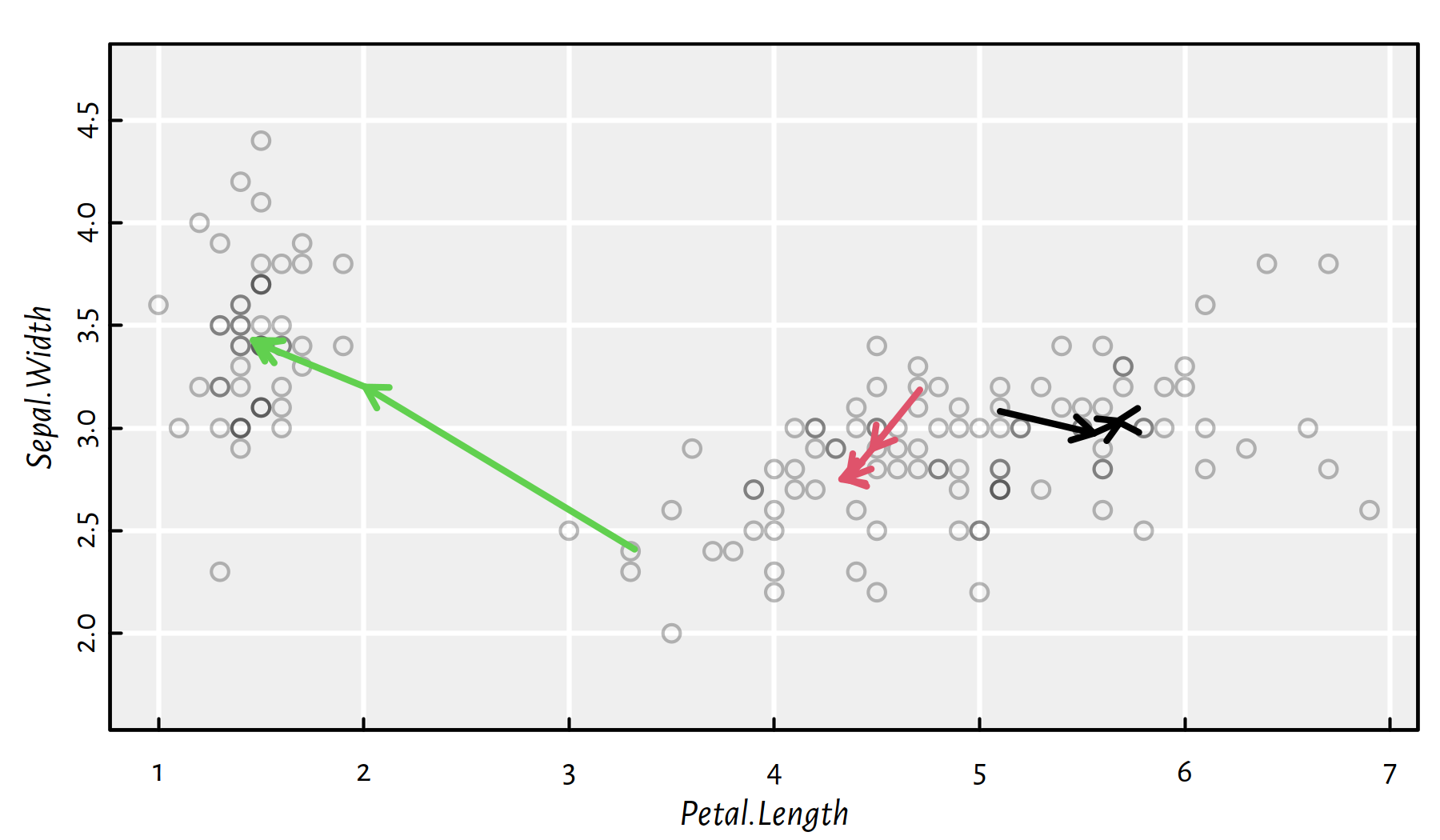
Figure 7.8: The arrows denote the cluster centres in each iteration of the Lloyd algorithm

On a side note, our algorithm needed 4 iterations to identify the (locally optimal) cluster centres. Figure 7.8 depicts its quest for the clustering grail.

7.3.1 Introduction

In K-means, we need to specify the number of clusters, \(K\), in advance. What if we don’t have any idea how to choose this parameter (which is often the case)?

Also, the problem with K-means is that there is no guarantee that a \(K\)-partition is any “similar” to the \(K'\)-one for \(K\neq K'\), see Figure 7.9.

km1 <- kmeans(X, 3, nstart=10)
km2 <- kmeans(X, 4, nstart=10)
plot(X, col=km1$cluster, pch=km2$cluster, asp=1)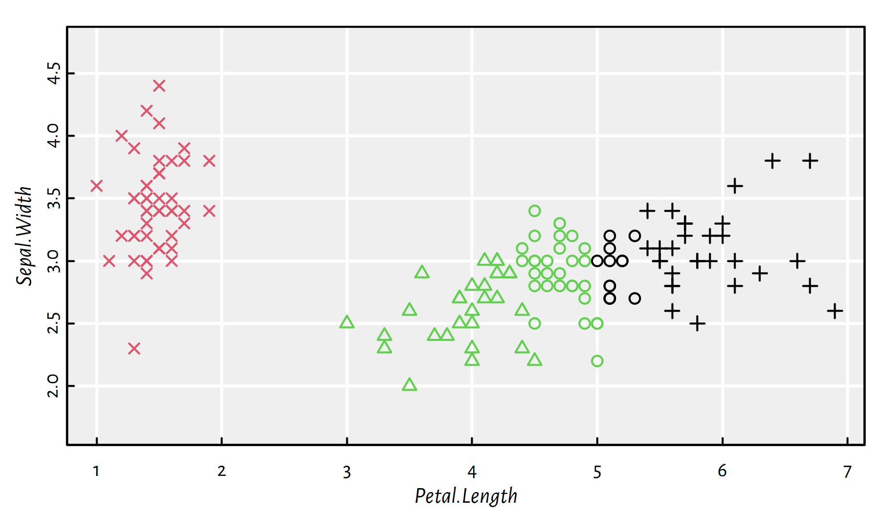

Figure 7.9: 3-means (colours) vs. 4-means (symbols) on example data; the “circle” cluster cannot decide if it likes the green or the black one more

Hierarchical methods, on the other hand, output a whole hierarchy of mutually nested partitions, which increase the interpretability of the results. A \(K\)-partition for any \(K\) can be extracted later at any time.

In this book we will be interested in agglomerative hierarchical algorithms:

• at the lowest level of the hierarchy, each point belongs to its own cluster (there are \(n\) singletons);

• at the highest level of the hierarchy, there is one cluster that embraces all the points;

• moving from the \(i\)-th to the \((i+1)\)-th level, we select (somehow; see below) a pair of clusters to be merged.

7.3.2 Example in R

The most basic implementation of a few agglomerative hierarchical clustering algorithms is provided by the hclust() function, which works on a pairwise distance matrix.

# Euclidean distances between all pairs of points:
D <- dist(X)
# Apply Complete Linkage (the default, details below):
h <- hclust(D) # method="complete"
print(h)

## 
## Call:
## hclust(d = D)
## 
## Cluster method   : complete 
## Distance         : euclidean 
## Number of objects: 150

Remark.

There are \(n(n-1)/2\) unique pairwise distances between \(n\) points. Don’t try calling dist() on large data matrices. Already \(n=100{,}000\) points consumes 40 GB of available memory (assuming that each distance is stored as an 8-byte double-precision floating point number); packages fastcluster and genieclust, among other, aim to solve this problem.

The obtained hierarchy (tree) can be cut at an arbitrary level by applying the cutree() function.

cutree(h, k=3) # extract the 3-partition

##  [1] 1 1 1 1 1 1 1 1 1 1 1 1 1 1 1 1 1 1 1 1 1 1 1 1 1 1 1 1 1 1 1 1 1 1
## [35] 1 1 1 1 1 1 1 1 1 1 1 1 1 1 1 1 2 2 2 2 2 2 2 2 2 2 2 2 2 2 2 2 2 2
## [69] 2 2 2 2 2 2 2 2 2 2 2 2 2 2 2 2 2 2 2 2 2 2 2 2 2 2 2 2 2 2 2
##  [ reached getOption("max.print") -- omitted 51 entries ]

The cuts of the hierarchy at different levels are depicted in Figure 7.10. The obtained 3-partition also matches the true Iris species quite well. However, now it makes total sense to “zoom” our partitioning in or out and investigate how are the subgroups decomposed or aggregated when we change \(K\).

par(mfrow=c(2,2))
plot(X, col=cutree(h, k=5), ann=FALSE)
legend("top", legend="k=5", bg="white")
plot(X, col=cutree(h, k=4), ann=FALSE)
legend("top", legend="k=4", bg="white")
plot(X, col=cutree(h, k=3), ann=FALSE)
legend("top", legend="k=3", bg="white")
plot(X, col=cutree(h, k=2), ann=FALSE)
legend("top", legend="k=2", bg="white")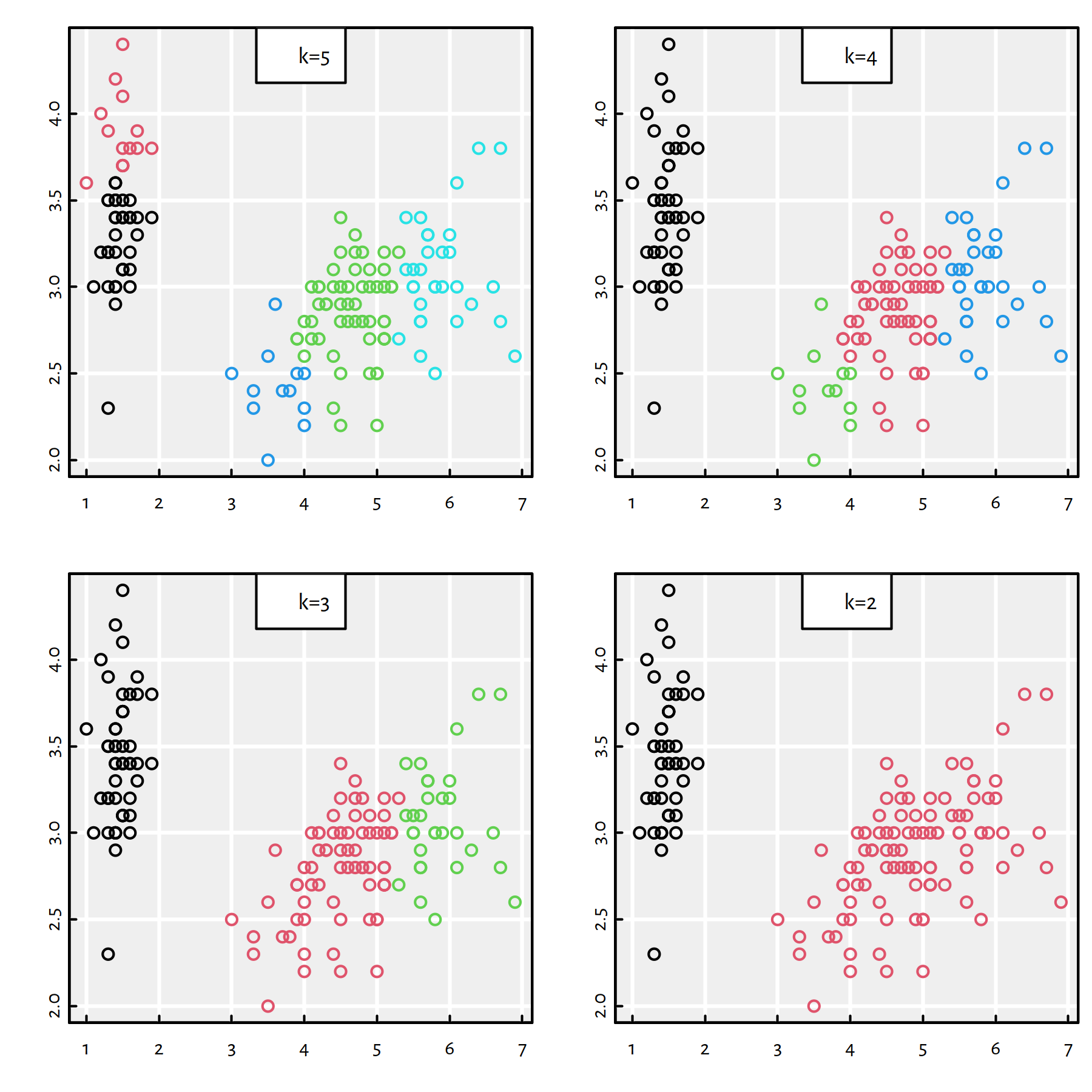

Figure 7.10: Complete linkage – 4 different cuts

7.3.3 Linkage Functions

Let’s formalise the clustering process. Initially, \(\mathcal{C}^{(0)}=\{\{\mathbf{x}_{1,\cdot}\},\dots,\{\mathbf{x}_{n,\cdot}\}\}\), i.e., each point is a member of its own cluster.

While an agglomerative hierarchical clustering algorithm is being computed, there are \(n-k\) clusters at the \(k\)-th step of the procedure, \(\mathcal{C}^{(k)}=\{C_1^{(k)},\dots,C_{n-k}^{(k)}\}\).

When proceeding from step \(k\) to \(k+1\), we determine the two groups \(C_u^{(k)}\) and \(C_v^{(k)}\), \(u<v\), to be merged together so that the clustering at the higher level is of the form: \[ \mathcal{C}^{(k+1)} = \left\{ C_1^{(k)},\dots,C_{u-1}^{(k)}, C_u^{(k)}{\cup C_v^{(k)}}, C_{u+1}^{(k)},\dots,C_{v-1}^{(k)}, C_{v+1}^{(k)},\dots,C_{n-k}^{(k)} \right\}. \]

Thus, \((\mathcal{C}^{(0)}, \mathcal{C}^{(1)}, \dots, \mathcal{C}^{(n-1)})\) form a sequence of nested partitions of the input dataset with the last level being just one big cluster, \(\mathcal{C}^{(n-1)}=\left\{ \{\mathbf{x}_{1,\cdot},\mathbf{x}_{2,\cdot},\dots,\mathbf{x}_{n,\cdot}\} \right\}\).

There is one component missing – how to determine the pair of clusters \(C_u^{(k)}\) and \(C_v^{(k)}\) to be merged with each other at the \(k\)-th iteration? Of course this will be expressed as some optimisation problem (although this time, a simple one)! The decision will be based on: \[ \mathrm{arg}\min_{u < v} d^*(C_u^{(k)}, C_v^{(k)}), \] where \(d^*(C_u^{(k)}, C_v^{(k)})\) is the distance between two clusters \(C_u^{(k)}\) and \(C_v^{(k)}\).

Note that we usually only consider the distances between individual points, not sets of points. Hence, \(d^*\) must be a suitable extension of a pointwise distance \(d\) (usually the Euclidean metric) to whole sets.

We will assume that \(d^*(\{\mathbf{x}_{i,\cdot}\},\{\mathbf{x}_{j,\cdot}\})= d(\mathbf{x}_{i,\cdot},\mathbf{x}_{j,\cdot})\), i.e., the distance between singleton clusters is the same as the distance between the points themselves. As far as more populous point groups are concerned, there are many popular choices of \(d^*\) (which in the context of hierarchical clustering we call linkage functions):

• single linkage:

  \[ d_\text{S}^*(C_u^{(k)}, C_v^{(k)}) = \min_{\mathbf{x}_{i,\cdot}\in C_u^{(k)}, \mathbf{x}_{j,\cdot}\in C_v^{(k)}} d(\mathbf{x}_{i,\cdot},\mathbf{x}_{j,\cdot}), \]

• complete linkage:

  \[ d_\text{C}^*(C_u^{(k)}, C_v^{(k)}) = \max_{\mathbf{x}_{i,\cdot}\in C_u^{(k)}, \mathbf{x}_{j,\cdot}\in C_v^{(k)}} d(\mathbf{x}_{i,\cdot},\mathbf{x}_{j,\cdot}), \]

• average linkage:

  \[ d_\text{A}^*(C_u^{(k)}, C_v^{(k)}) = \frac{1}{|C_u^{(k)}| |C_v^{(k)}|} \sum_{\mathbf{x}_{i,\cdot}\in C_u^{(k)}}\sum_{\mathbf{x}_{j,\cdot}\in C_v^{(k)}} d(\mathbf{x}_{i,\cdot},\mathbf{x}_{j,\cdot}). \]

An illustration of the way different linkages are computed is given in Figure 7.11.

Figure 7.11: In single linkage, we find the closest pair of points; in complete linkage, we seek the pair furthest away from each other; in average linkage, we determine the arithmetic mean of all pairwise distances

Assuming \(d_\text{S}^*\), \(d_\text{C}^*\) or \(d_\text{A}^*\) in the aforementioned procedure leads to single, complete or average linkage-based agglomerative hierarchical clustering algorithms, respectively (referred to as single linkage etc. for brevity).

hs <- hclust(D, method="single")
hc <- hclust(D, method="complete")
ha <- hclust(D, method="average")

Figure 7.12 compares the 5-, 4- and 3-partitions obtained by applying the 3 above linkages. Note that it’s in very nature of the single linkage algorithm that it’s highly sensitive to outliers.

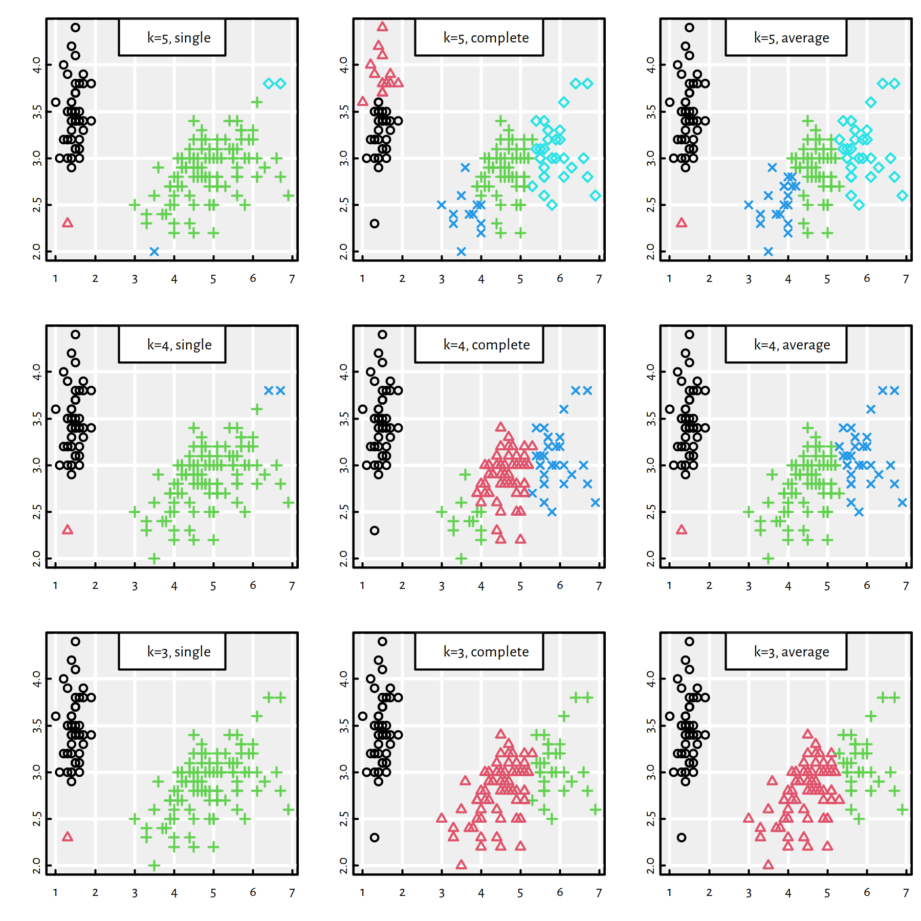
Figure 7.12: 3 cuts of 3 different hierarchies

7.3.4 Cluster Dendrograms

A dendrogram (which we can plot by calling plot(h), where h is the result returned by hclust()) depicts the distances (as defined by the linkage function) between the clusters merged at every stage of the agglomerative procedure. This can provide us with some insight into the underlying data structure as well as with hits about at which level the tree could be cut.

Figure 7.13 depicts the three dendrograms that correspond to the clusterings obtained by applying different linkages. Each tree has 150 leaves (at the bottom) that represent the 150 points in our example dataset. Each “edge” (joint) represents a group of points being merged. For instance, the very top joint in the middle subfigure is located at height of \(\simeq 6\), which is exactly the maximal pairwise distance (complete linkage) between the points in the last two last clusters.

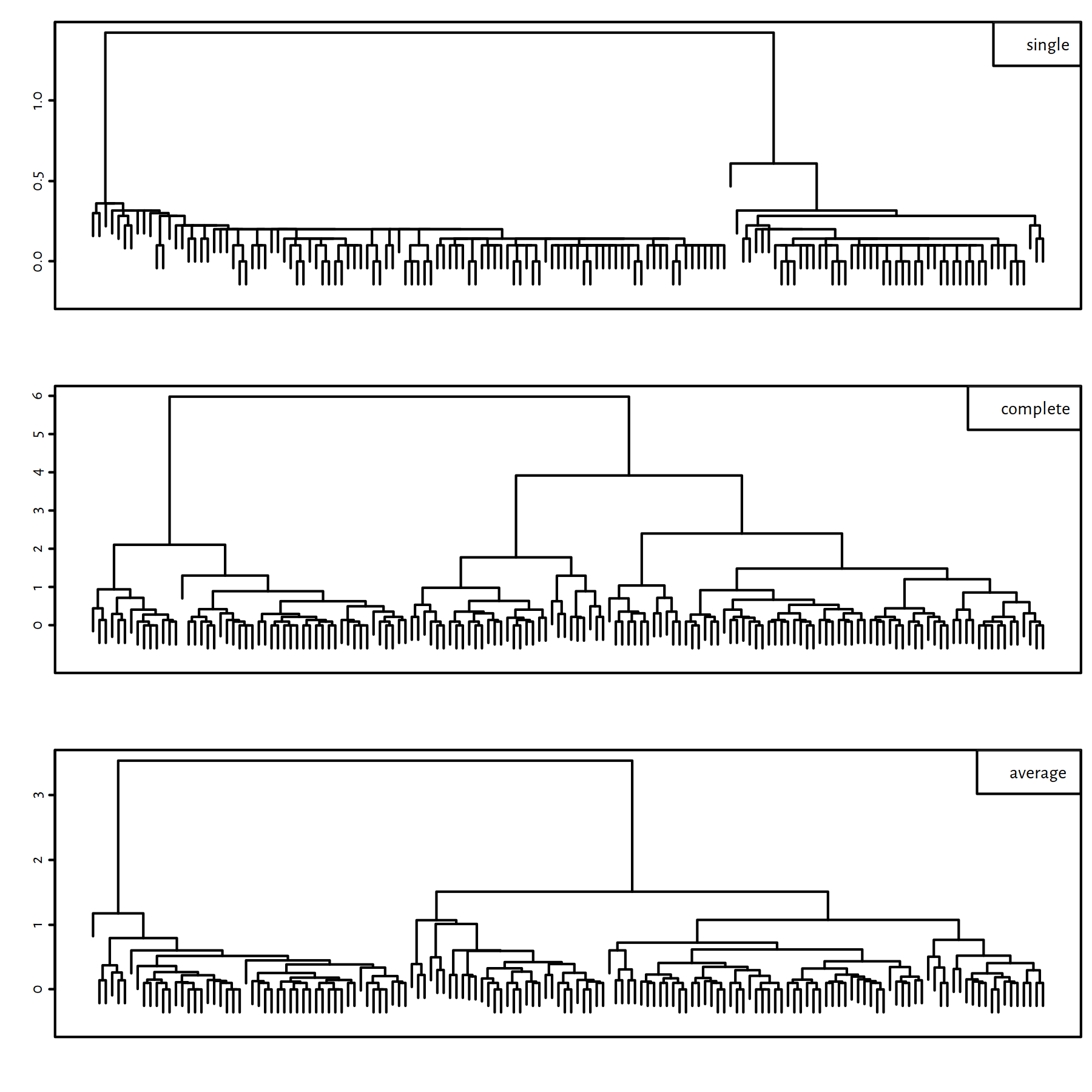
Figure 7.13: Cluster dendrograms for the single, complete and average linkages

7.4.1 Clustering of the World Factbook

Let’s perform a cluster analysis of countries based on the information contained in the World Factbook dataset:

factbook <- read.csv("datasets/world_factbook_2020.csv",
    comment.char="#")

count_na_in_columns <- sapply(factbook, function(x) sum(is.na(x)))
factbook <- factbook[count_na_in_columns <= 40] # column removal

factbook <- na.omit(factbook) # row removal
dim(factbook) # how many rows and cols remained

## [1] 203  23

for (i in 2:ncol(factbook)) # skip `country`
    factbook[[i]] <- (factbook[[i]]-mean(factbook[[i]]))/
                        sd(factbook[[i]])

km <- kmeans(factbook[-1], 2, nstart=10)

km_countries <- split(factbook[[1]], km$cluster)
km_countries[[1]]

## [1] "China"         "India"         "United States"

t(km$centers) # transposed for readability

##                                        1          2
## area                            3.661581 -0.0549237
## population                      6.987279 -0.1048092
## median_age                      0.477991 -0.0071699
## population_growth_rate         -0.252774  0.0037916
## birth_rate                     -0.501030  0.0075155
## death_rate                      0.153915 -0.0023087
## net_migration_rate              0.236449 -0.0035467
## infant_mortality_rate          -0.139577  0.0020937
## life_expectancy_at_birth        0.251541 -0.0037731
## total_fertility_rate           -0.472716  0.0070907
## gdp_purchasing_power_parity     7.213681 -0.1082052
## gdp_real_growth_rate            0.369499 -0.0055425
## gdp_per_capita_ppp              0.298103 -0.0044715
## labor_force                     6.914319 -0.1037148
## taxes_and_other_revenues       -0.922735  0.0138410
## budget_surplus_or_deficit      -0.012627  0.0001894
## inflation_rate_consumer_prices -0.096626  0.0014494
## exports                         5.341178 -0.0801177
## imports                         5.956538 -0.0893481
## telephones_fixed_lines          5.989858 -0.0898479
## internet_users                  6.997126 -0.1049569
## airports                        4.551832 -0.0682775

Click here for a solution.

Recall that the complete linkage-based method is implemented in the hclust() function:

d <- dist(factbook[-1]) # skip `country`
h <- hclust(d, method="complete")

A “nice” number of clusters to divide our dataset into can be read from the dendrogram, see Figure 7.14.

plot(h, labels=FALSE, ann=FALSE); box()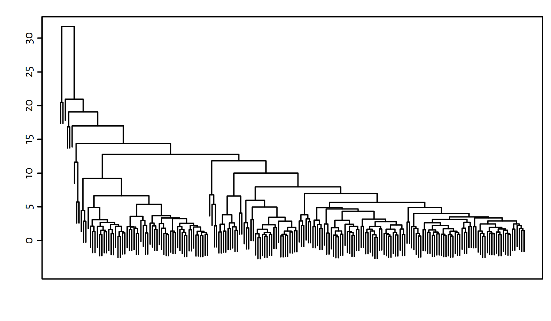

Figure 7.14: Cluster dendrogram for the World Factbook dataset – Complete linkage

It seems that a 9-partition might reveal something interesting, because it will distinguish two larger country groups. However, there will be many singletons if we do so either way.

y <- cutree(h, 9)
h_countries <- split(factbook[[1]], y)
sapply(h_countries, length) # number of elements in each cluster

##   1   2   3   4   5   6   7   8   9 
## 138  56   1   1   3   1   1   1   1

Most likely this is not an interesting partitioning of this dataset, therefore we’ll not be exploring it any further.

Click here for a solution.

The Genie algorithm (Gagolewski et al. 2016) is a hierarchical clustering algorithm implemented in R package genieclust. It’s interface is compatible with hclust().

library("genieclust")
d <- dist(factbook[-1])
g <- gclust(d)

The cluster dendrogram in Figure 7.15 reveals 3 evident clusters.

plot(g, labels=FALSE, ann=FALSE); box()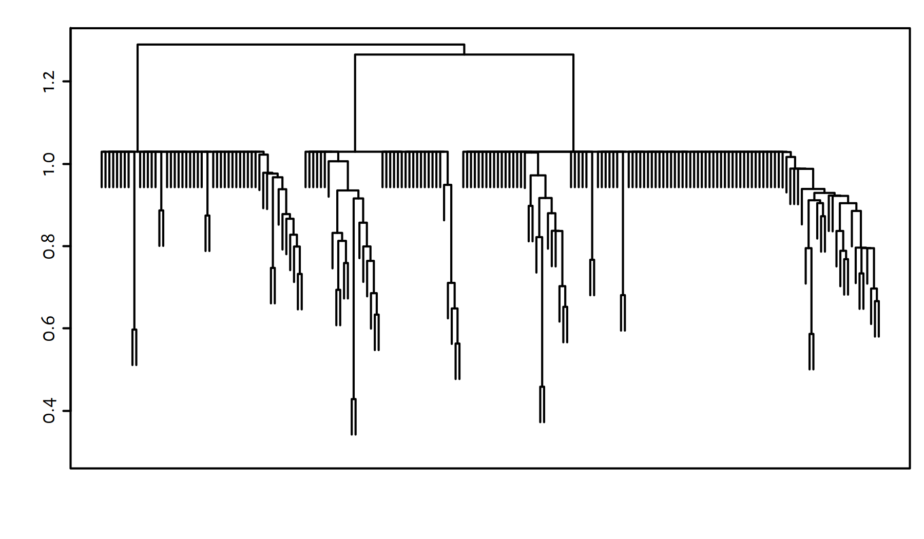

Figure 7.15: Cluster dendrogram for the World Factbook dataset – Genie algorithm

Let’s determine the 3-partition of the data set.

y <- cutree(g, 3)

Here are few countries in each cluster:

y <- cutree(g, 3)
sapply(split(factbook$countr, y), sample, 6)

##      1                    2                                  
## [1,] "Dominican Republic" "Congo, Republic of the"           
## [2,] "Venezuela"          "Sao Tome and Principe"            
## [3,] "Sri Lanka"          "Tanzania"                         
## [4,] "Malta"              "Botswana"                         
## [5,] "China"              "Congo, Democratic Republic of the"
## [6,] "Tajikistan"         "Malawi"                           
##      3             
## [1,] "Lithuania"   
## [2,] "Portugal"    
## [3,] "Korea, South"
## [4,] "Bulgaria"    
## [5,] "Germany"     
## [6,] "Moldova"

We can draw the countries in each cluster on a map by using the rworldmap package (see its documentation for more details), see Figure 7.16.

library("rworldmap")
library("RColorBrewer")
mapdata <- data.frame(country=factbook$country, cluster=y)
# 3 country names must be adjusted to get a match
mapdata$country[mapdata$country == "Czechia"] <- "Czech Republic"
mapdata$country[mapdata$country == "Eswatini"] <- "Swaziland"
mapdata$country[mapdata$country == "Cabo Verde"] <- "Cape Verde"
mapdata <- joinCountryData2Map(mapdata, joinCode="NAME",
  nameJoinColumn="country")

## 203 codes from your data successfully matched countries in the map
## 0 codes from your data failed to match with a country code in the map
## 40 codes from the map weren't represented in your data

par(mar=c(0,0,0,0))
mapCountryData(mapdata, nameColumnToPlot="cluster",
    catMethod="categorical", missingCountryCol="gray",
    colourPalette=brewer.pal(3, "Set1"),
    mapTitle="", addLegend=TRUE)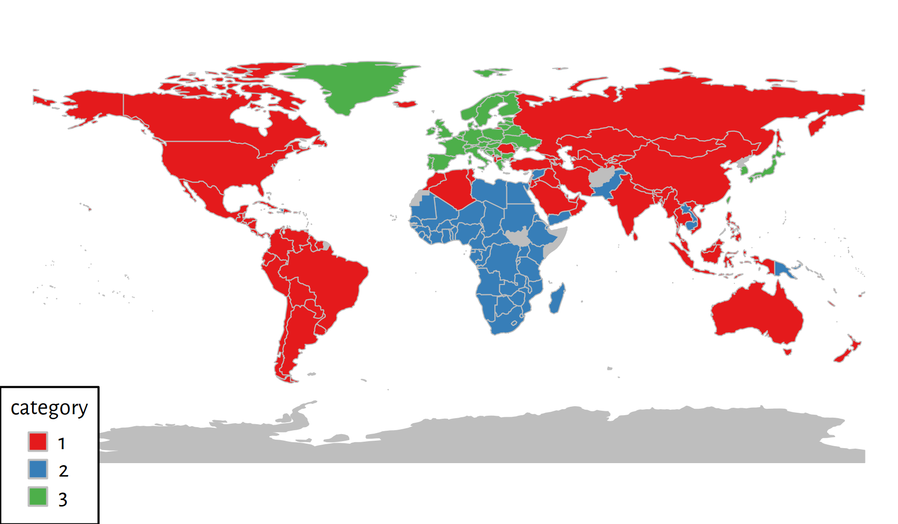

Figure 7.16: 3 clusters discovered by the Genie algorithm

Here are the average Z-scores in each cluster:

round(sapply(split(factbook[-1], y), colMeans), 3)

##                                     1      2      3
## area                            0.124 -0.068 -0.243
## population                      0.077 -0.058 -0.130
## median_age                      0.118 -1.219  1.261
## population_growth_rate         -0.227  1.052 -0.757
## birth_rate                     -0.316  1.370 -0.930
## death_rate                     -0.439  0.071  1.075
## net_migration_rate             -0.123  0.053  0.260
## infant_mortality_rate          -0.366  1.399 -0.835
## life_expectancy_at_birth        0.354 -1.356  0.812
## total_fertility_rate           -0.363  1.332 -0.758
## gdp_purchasing_power_parity     0.084 -0.213  0.052
## gdp_real_growth_rate           -0.062  0.126  0.002
## gdp_per_capita_ppp              0.021 -0.744  0.905
## labor_force                     0.087 -0.096 -0.107
## taxes_and_other_revenues       -0.095 -0.584  1.006
## budget_surplus_or_deficit      -0.113 -0.188  0.543
## inflation_rate_consumer_prices  0.044 -0.013 -0.099
## exports                        -0.013 -0.318  0.447
## imports                         0.007 -0.308  0.379
## telephones_fixed_lines          0.048 -0.244  0.186
## internet_users                  0.093 -0.178 -0.016
## airports                        0.104 -0.131 -0.107

That is really interesting! The interpretation of the above is left to the reader.

7.4.2 Unbalance Dataset – K-Means Needs Multiple Starts

Let us consider a benchmark (artificial) dataset proposed in (Rezaei & Fränti 2016):

unbalance <- as.matrix(read.csv("datasets/sipu_unbalance.csv",
    header=FALSE, sep=" ", comment.char="#"))
unbalance <- unbalance/10000-30 # a more user-friendly scale

According to its authors, this dataset is comprised of 8 clusters: there are 3 groups on the lefthand side (2000 points each) and 5 on the right side (100 each).

plot(unbalance, asp=1)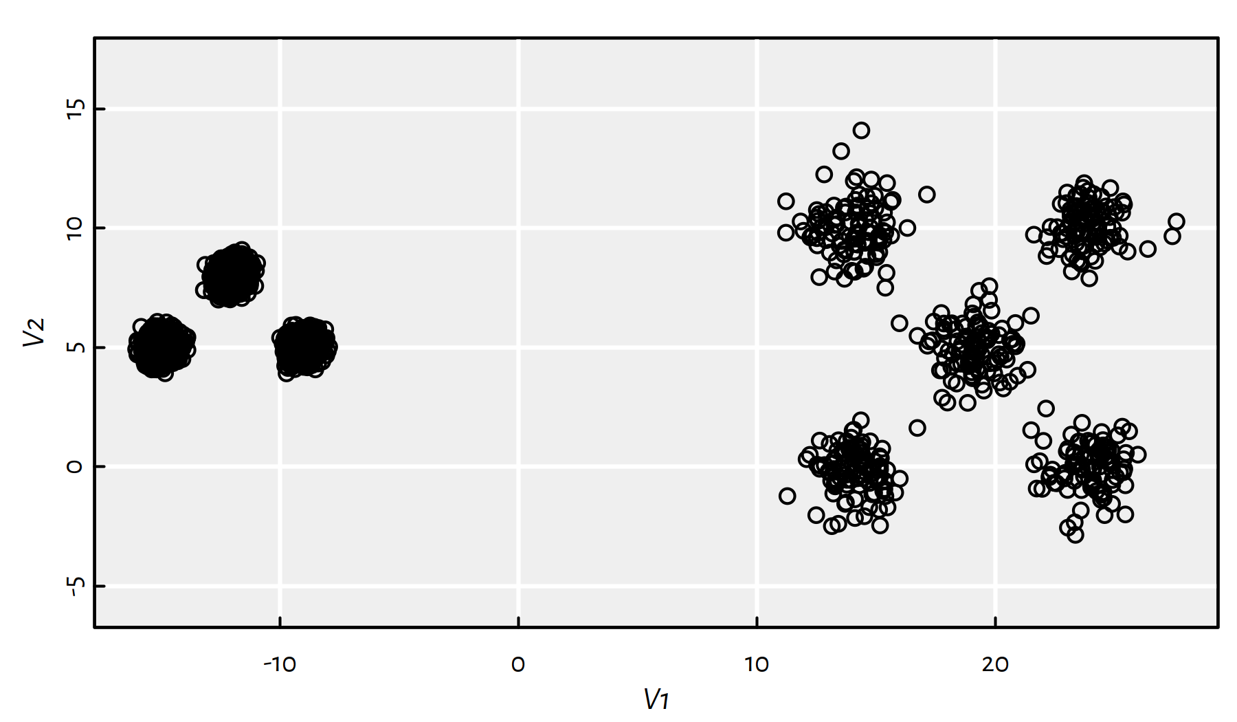

(#fig:sipu_unbalance2) sipu_unbalance dataset

Click here for a solution.

Of course, here by “the” K-means we mean the default method available in the kmeans() function. The clustering results are depicted in Figure 7.17.

km <- kmeans(unbalance, 8, nstart=10)
plot(unbalance, asp=1, col=km$cluster)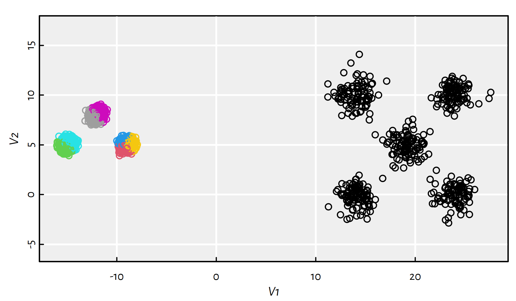

Figure 7.17: Results of K-means on the sipu_unbalance dataset

This is far from what we expected. The total within-cluster distances are equal to:

km$tot.withinss

## [1] 21713

Increasing the number of restarts even further improves the solution, but the local minimum is still far from the global one, compare Figure 7.18.

km <- suppressWarnings(kmeans(unbalance, 8, nstart=1000, iter.max=1000))
plot(unbalance, asp=1, col=km$cluster)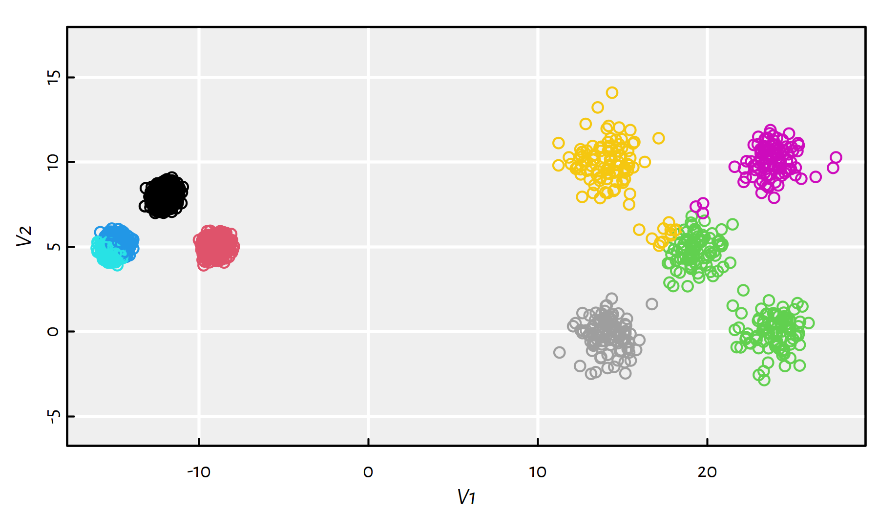

Figure 7.18: Results of K-means on the sipu_unbalance dataset – many more restarts

km$tot.withinss

## [1] 4378

Click here for a solution.

Clustering is – in its essence – an unsupervised learning method, so what we’re going to do now could be called, let’s be blunt about it, cheating. Luckily, we have an oracle at our disposal – it has provided us with the following educated guesses (by looking at the scatter plot) about the localisation of the cluster centres:

cntr <- matrix(ncol=2, byrow=TRUE, c(
   -15,   5,
   -12,   10,
   -10,   5,
    15,   0,
    15,   10,
    20,   5,
    25,   0,
    25,   10))

Running kmeans() yields the clustering depicted in Figure 7.19.

km <- kmeans(unbalance, cntr)
plot(unbalance, asp=1, col=km$cluster)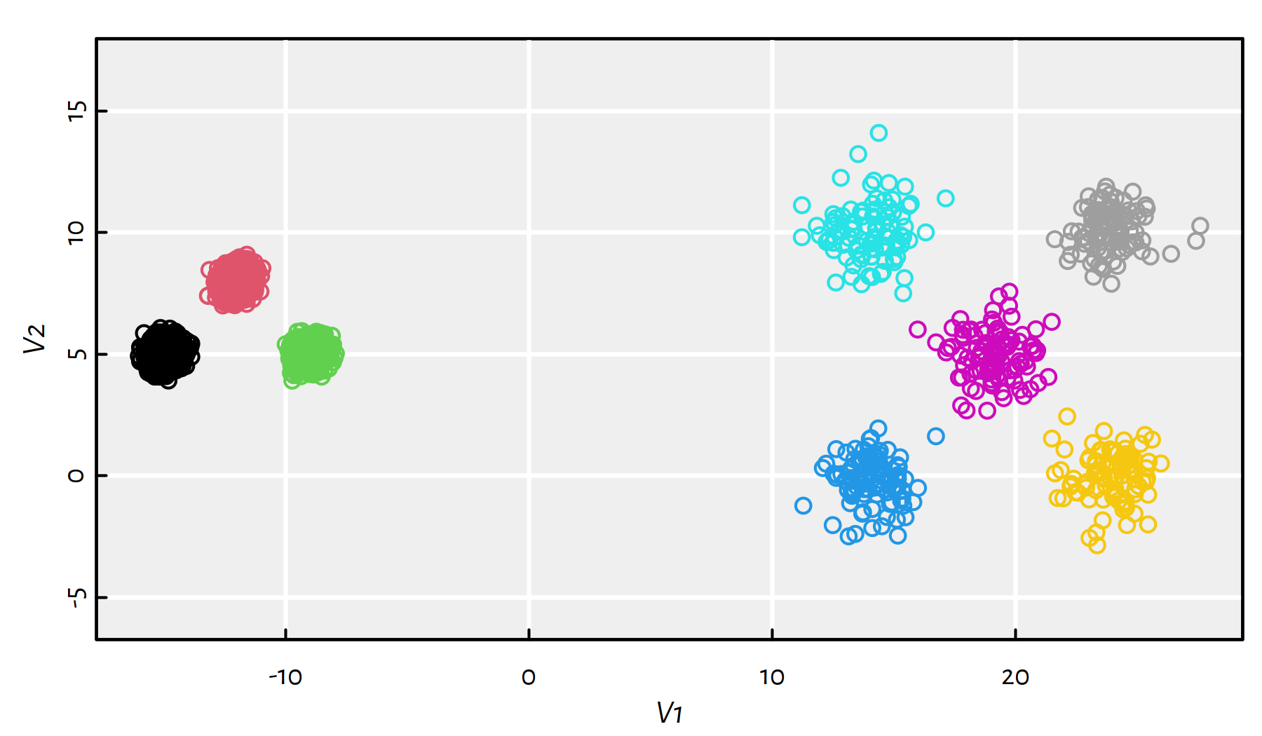

Figure 7.19: Results of K-means on the sipu_unbalance dataset – an educated guess on the cluster centres’ locations

The total within-cluster distances are now equal to:

km$tot.withinss

## [1] 2144.9

This is finally the globally optimal solution to the K-means problem we were asked to solve. Recall that the algorithms implemented in the kmeans() function are just fast heuristics that are supposed to find local optima of the K-means objective function, which is given by the within-cluster sum of squared Euclidean distances.

7.4.3 Clustering of Typical 2D Benchmark Datasets

Let us consider a few clustering benchmark datasets available at https://github.com/gagolews/clustering_benchmarks_v1 and http://cs.joensuu.fi/sipu/datasets/. Here is a list of file names together with the corresponding numbers of clusters (as given by datasets’ authors):

files <- c("datasets/wut_isolation.csv",
           "datasets/wut_mk2.csv",
           "datasets/wut_z3.csv",
           "datasets/sipu_aggregation.csv",
           "datasets/sipu_pathbased.csv",
           "datasets/sipu_unbalance.csv")
Ks <- c(3, 2, 4, 7, 3, 8)

All the datasets are two-dimensional, hence we’ll be able to visualise the obtained results and assess the sensibility of the obtained clusterings.

Click here for a solution.

Apart from a call to the Genie algorithm with the default parameters, we will also look at the results it generates when we set giniThreshold of 0.5.

The following function is our workhorse that will perform all the computations and will draw all the figures for a single dataset:

clusterise <- function(file, K) {
    X <- read.csv(file,
        header=FALSE, sep=" ", comment.char="#")
    d <- dist(X)
    par(mfrow=c(2, 3))
    par(mar=c(0.5, 0.5, 2, 0.5))

    y <- kmeans(X, K, nstart=10)$cluster
    plot(X, asp=1, col=y, ann=FALSE, axes=FALSE)
    mtext("K-means", line=0.5)

    y <- cutree(hclust(d, "complete"), K)
    plot(X, asp=1, col=y, ann=FALSE, axes=FALSE)
    mtext("Complete Linkage", line=0.5)

    y <- cutree(hclust(d, "average"), K)
    plot(X, asp=1, col=y, ann=FALSE, axes=FALSE)
    mtext("Average Linkage", line=0.5)

    y <- cutree(hclust(d, "single"), K)
    plot(X, asp=1, col=y, ann=FALSE, axes=FALSE)
    mtext("Single Linkage", line=0.5)

    y <- cutree(genieclust::gclust(d), K) # gini_threshold=0.3
    plot(X, asp=1, col=y, ann=FALSE, axes=FALSE)
    mtext("Genie (default)", line=0.5)

    y <- cutree(genieclust::gclust(d, gini_threshold=0.5), K)
    plot(X, asp=1, col=y, ann=FALSE, axes=FALSE)
    mtext("Genie (g=0.5)", line=0.5)
}

Applying the above as clusterise(files[i], Ks[i]) yields Figures 7.20-7.25.

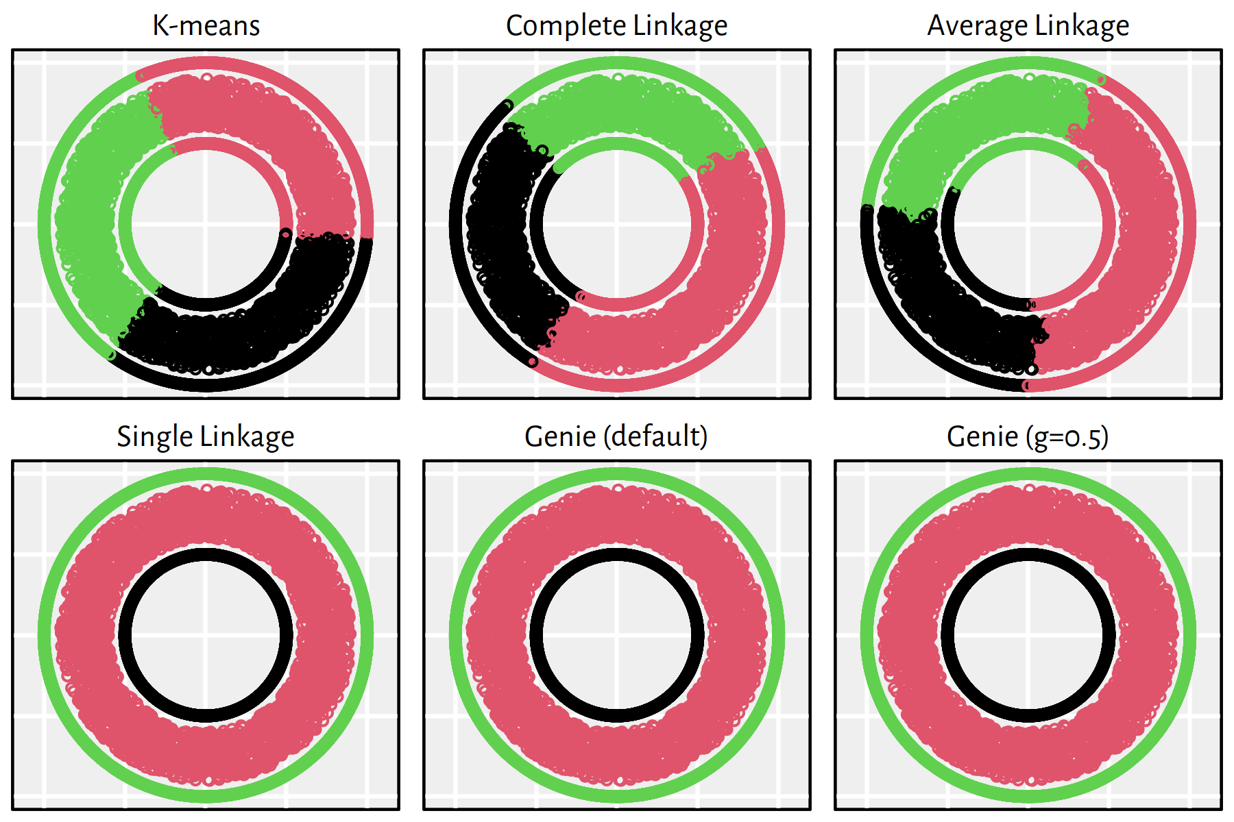
Figure 7.20: Clustering of the wut_isolation dataset

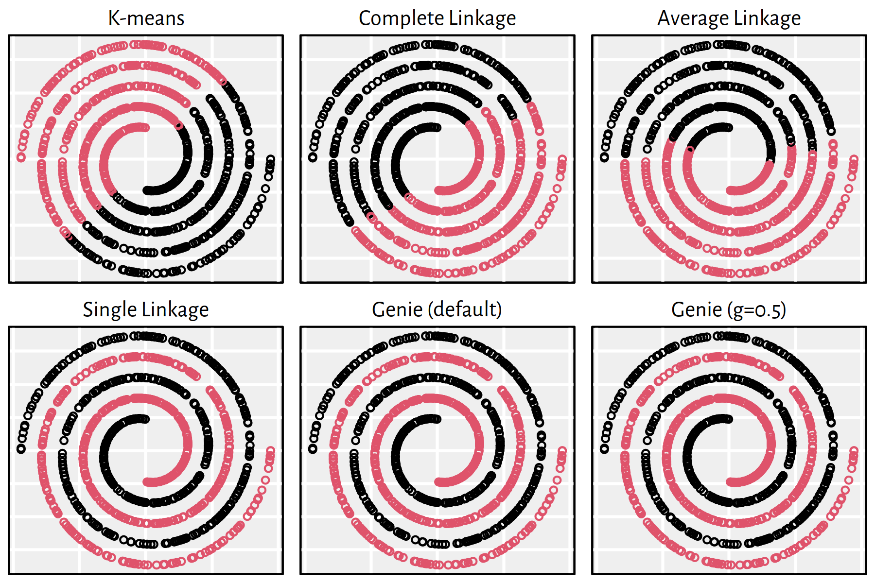
Figure 7.21: Clustering of the wut_mk2 dataset

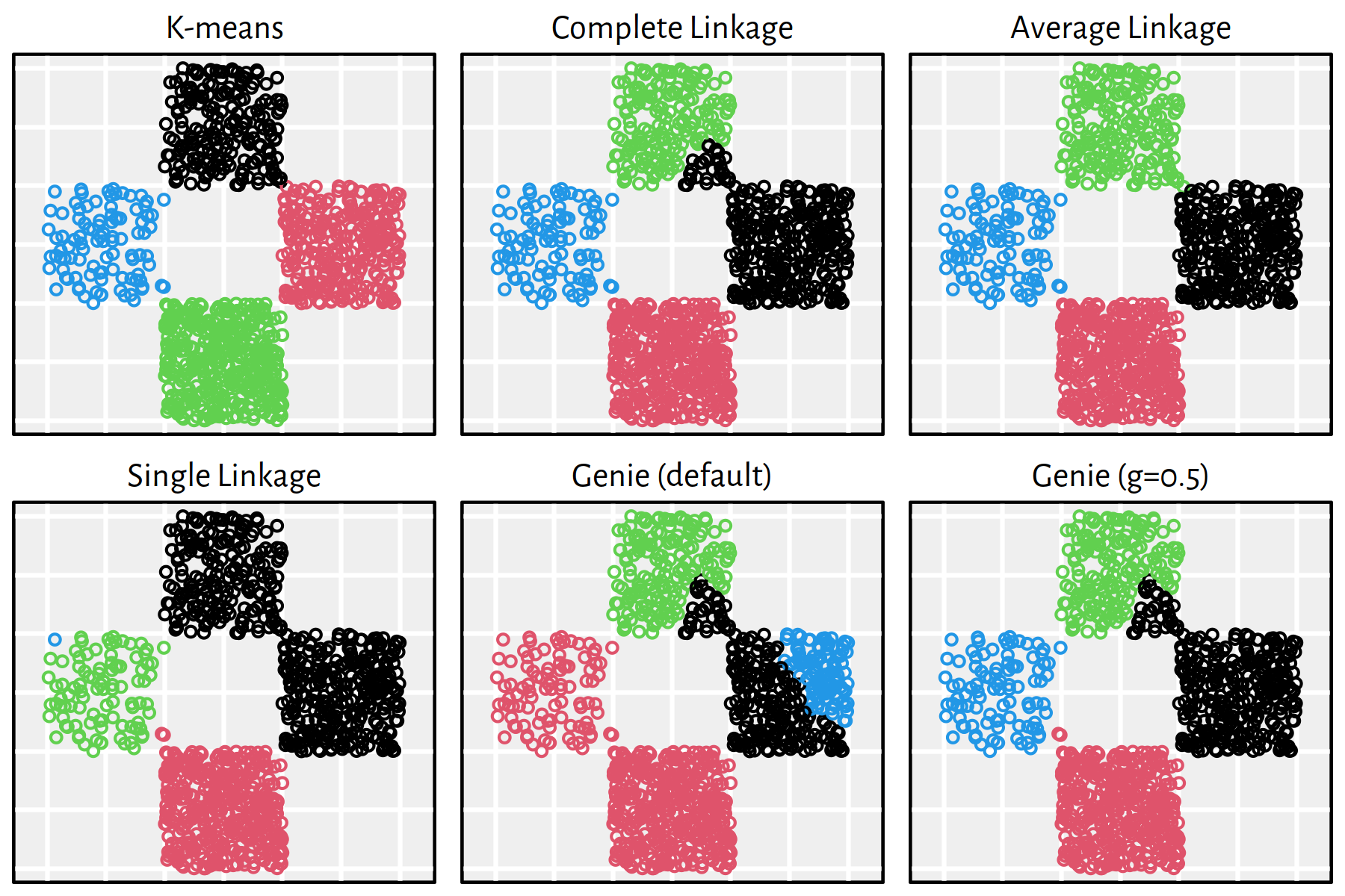
Figure 7.22: Clustering of the wut_z3 dataset

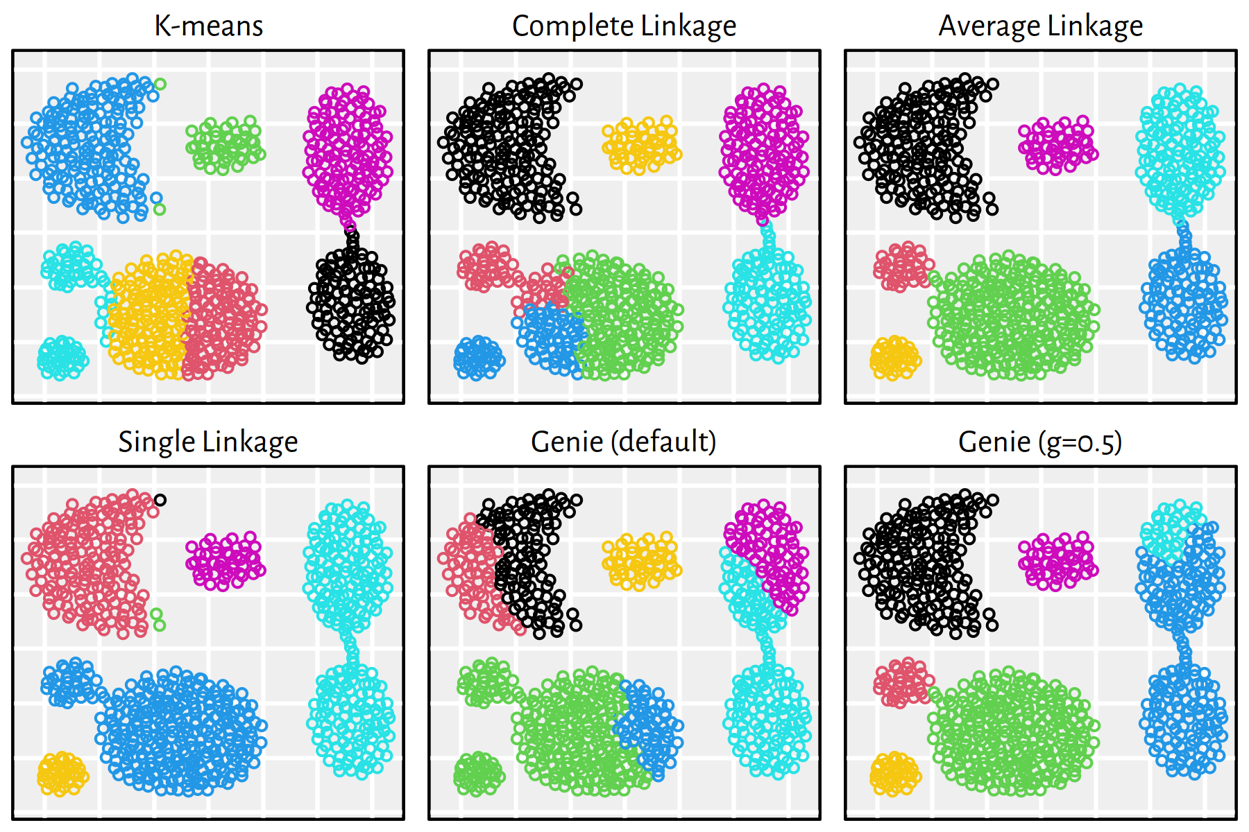
Figure 7.23: Clustering of the sipu_aggregation dataset

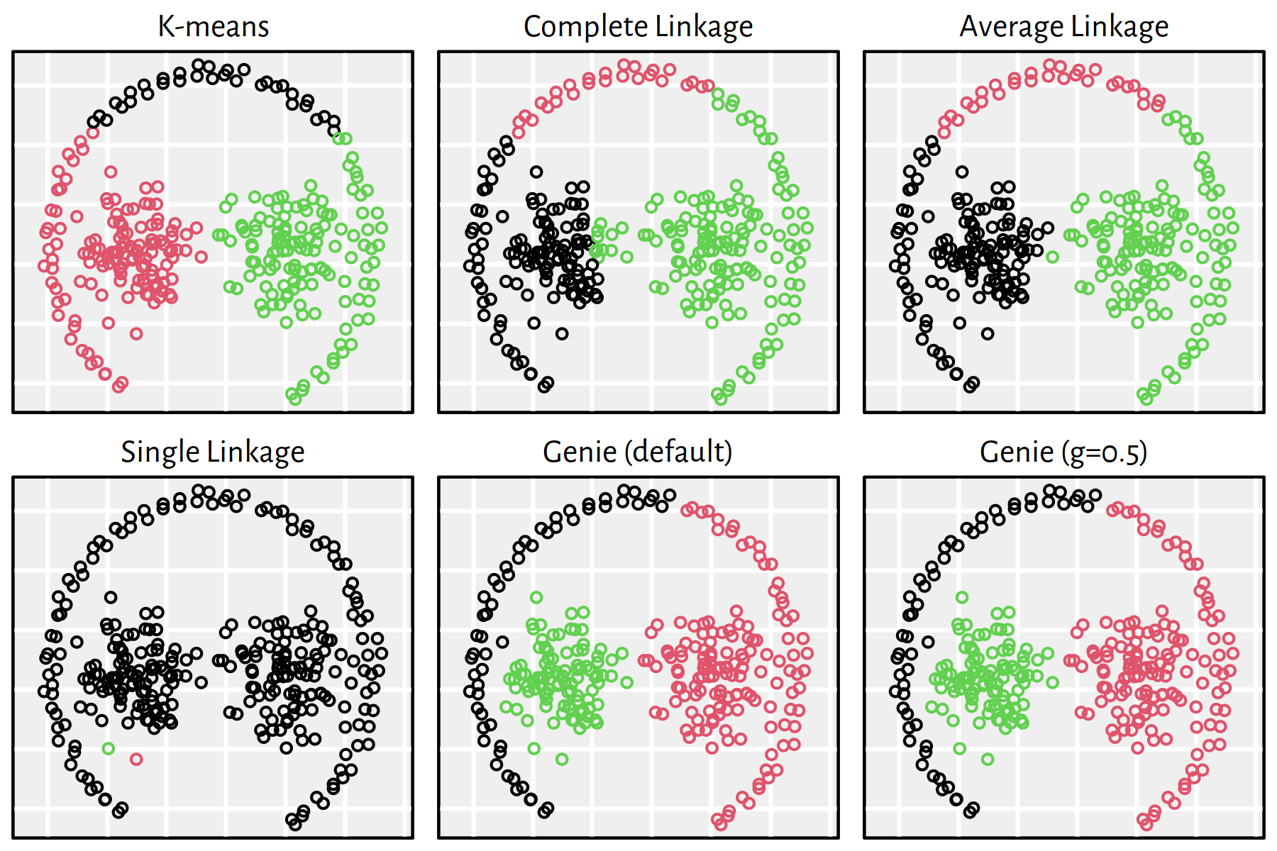
Figure 7.24: Clustering of the sipu_pathbased dataset

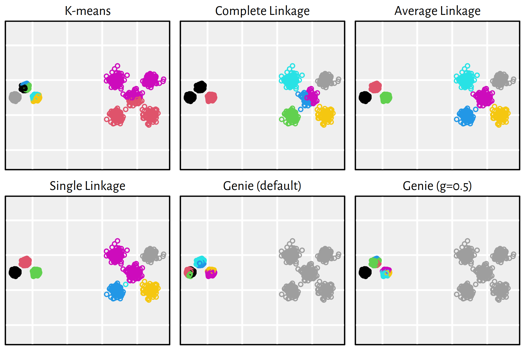
Figure 7.25: Clustering of the sipu_unbalance dataset

Note that, by definition, K-means is only able to detect clusters of convex shapes. The Genie algorithm, on the other hand, might fail to detect clusters of very small sizes amongst the more populous ones. Single linkage is very sensitive to outliers in data – it often outputs clusters of cardinality 1.

7.5.1 Remarks

Unsupervised learning is often performed during the data pre-processing and exploration stage. Assessing the quality of clustering is particularly challenging as, unlike in a supervised setting, we have no access to “ground truth” information.

In practice, we often apply different clustering algorithms and just see where they lead us. There’s no teacher that would tell us what we should do, so whatever we do is awesome, right? Well, not precisely. Most frequently, you, my dear reader, will work for some party that’s genuinely interested in your explaining why did you spent the last month coming up with nothing useful at all. Thus, the main body of work related to proving the use-full/less-ness will be on you.

Clustering methods can aid us in supervised tasks – instead of fitting a single “large model”, it might be useful to fit separate models to each cluster.

To sum up, the aim of K-means is to find \(K\) clusters based on the notion of the points’ closeness to the cluster centres. Remember that \(K\) must be set in advance. By definition (* via its relation to Voronoi diagrams), all clusters will be of convex shapes.

However, we may try applying \(K'\)-means for \(K' \gg K\) to obtain a “fine grained” compressed representation of data and then combine the (sub)clusters into more meaningful groups using other methods (such as the hierarchical ones).

Iterative K-means algorithms are very fast (e.g., a mini-batch version of the algorithm can be implement to speed up the optimisation process) even for large data sets, but they may fail to find a desirable solution, especially if clusters are unbalanced.

Hierarchical methods, on the other hand, output a whole family of mutually nested partitions, which may provide us with insight into the underlying structure of data data. Unfortunately, there is no easy way to assign new points to existing clusters; yet, you can always build a classifier (e.g., a decision tree or a neural network) that learns the discovered labels.

A linkage scheme must be chosen with care, for instance, single linkage can be sensitive to outliers. However, it is generally the fastest. The methods implemented in hclust() are generally slow; they have time complexity between \(O(n^2)\) and \(O(n^3)\).

Remark.

Note that the fastcluster package provides a more efficient and memory-saving implementation of some methods available via a call to hclust(). See also the genieclust package for a super-robust version of the single linkage algorithm based on the datasets’s Euclidean minimum spanning tree, which can be computed quite quickly.

Finally, note that all the discussed clustering methods are based on the notion of pairwise distances. These of course tend to behave weirdly in high-dimensional spaces (“the curse of dimensionality”). Moreover, some hardcore feature engineering might be needed to obtain meaningful results.

7.5.2 Further Reading

Recommended further reading: (James et al. 2017: Section 10.3)

Other: (Hastie et al. 2017: Section 14.3)

Additionally, check out other noteworthy clustering approaches:

• Genie (see R package genieclust) (Gagolewski et al. 2016, Cena & Gagolewski 2020)
• ITM (Müller et al. 2012)
• DBSCAN, HDBSCAN* (Ling 1973, Ester et al. 1996, Campello et al. 2015)
• K-medoids, K-medians
• Fuzzy C-means (a.k.a. weighted K-means) (Bezdek et al. 1984)
• Spectral clustering; e.g., (Ng et al. 2001)
• BIRCH (Zhang et al. 1996)