D Matrix Algebra in R

D.1.1 matrix()

A matrix can be created – amongst others – with a call to the matrix() function.

(A <- matrix(c(1, 2, 3, 4, 5, 6), byrow=TRUE, nrow=2))

##      [,1] [,2] [,3]
## [1,]    1    2    3
## [2,]    4    5    6

class(A)

## [1] "matrix" "array"

Given a numeric vector of length 6, we’ve asked R to convert to a numeric matrix with 2 rows (the nrow argument). The number of columns has been deduced automatically (otherwise, we would additionally have to pass ncol=3 to the function).

Using mathematical notation, above we have defined \(\mathbf{A}\in\mathbb{R}^{2\times 3}\):

\[ \mathbf{A}= \left[ \begin{array}{ccc} a_{1,1} & a_{1,2} & a_{1,3} \\ a_{2,1} & a_{2,2} & a_{2,3} \\ \end{array} \right] = \left[ \begin{array}{ccc} 1 & 2 & 3 \\ 4 & 5 & 6 \\ \end{array} \right] \]

We can fetch the size of the matrix by calling:

dim(A) # number of rows, number of columns

## [1] 2 3

We can also “promote” a “flat” vector to a column vector, i.e., a matrix with one column by calling:

as.matrix(1:3)

##      [,1]
## [1,]    1
## [2,]    2
## [3,]    3

D.1.2 Stacking Vectors

Other ways to create a matrix involve stacking a couple of vectors of equal lengths along each other:

rbind(1:3, 4:6, 7:9) # row bind

##      [,1] [,2] [,3]
## [1,]    1    2    3
## [2,]    4    5    6
## [3,]    7    8    9

cbind(1:3, 4:6, 7:9) # column bind

##      [,1] [,2] [,3]
## [1,]    1    4    7
## [2,]    2    5    8
## [3,]    3    6    9

These functions also allow for adding new rows/columns to existing matrices:

rbind(A, c(-1, -2, -3))

##      [,1] [,2] [,3]
## [1,]    1    2    3
## [2,]    4    5    6
## [3,]   -1   -2   -3

cbind(A, c(-1, -2))

##      [,1] [,2] [,3] [,4]
## [1,]    1    2    3   -1
## [2,]    4    5    6   -2

D.1.3 Beyond Numeric Matrices

Note that logical matrices are possible as well. For instance, knowing that comparison such as < and == are performed elementwise also in the case of matrices, we can obtain:

A >= 3

##       [,1]  [,2] [,3]
## [1,] FALSE FALSE TRUE
## [2,]  TRUE  TRUE TRUE

Moreover, although much more rarely used, we can define character matrices:

matrix(LETTERS[1:12], ncol=6)

##      [,1] [,2] [,3] [,4] [,5] [,6]
## [1,] "A"  "C"  "E"  "G"  "I"  "K" 
## [2,] "B"  "D"  "F"  "H"  "J"  "L"

D.1.4 Naming Rows and Columns

Just like vectors could be equipped with names attribute:

c(a=1, b=2, c=3)

## a b c 
## 1 2 3

matrices can be assigned row and column labels in the form of a list of two character vectors:

dimnames(A) <- list(
    c("a", "b"),     # row labels
    c("x", "y", "z") # column labels
)
A

##   x y z
## a 1 2 3
## b 4 5 6

D.1.5 Other Methods

The read.table() (and its special case, read.csv()), can be used to read a matrix from a text file. We will cover it in the next chapter, because technically it returns a data frame object (which we can convert to a matrix with a call to as.matrix()).

outer() applies a given (vectorised) function on each pair of elements from two vectors, forming a two-dimensional “grid”. More precisely outer(x, y, f, ...) returns a matrix \(\mathbf{Z}\) with length(x) rows and length(y) columns such that \(z_{i,j}=f(x_i, y_j, ...)\), where ... are optional further arguments to f.

outer(c(1, 10, 100), 1:5, "*") # apply the multiplication operator

##      [,1] [,2] [,3] [,4] [,5]
## [1,]    1    2    3    4    5
## [2,]   10   20   30   40   50
## [3,]  100  200  300  400  500

outer(c("A", "B"), 1:8, paste, sep="-") # concatenate strings

##      [,1]  [,2]  [,3]  [,4]  [,5]  [,6]  [,7]  [,8] 
## [1,] "A-1" "A-2" "A-3" "A-4" "A-5" "A-6" "A-7" "A-8"
## [2,] "B-1" "B-2" "B-3" "B-4" "B-5" "B-6" "B-7" "B-8"

simplify2array() is an extension of the unlist() function. Given a list of vectors, each of length one, it will return an “unlisted” vector. However, if a list of equisized vectors of greater lengths is given, these will be converted to a matrix.

simplify2array(list(1, 11, 21))

## [1]  1 11 21

simplify2array(list(1:3, 11:13, 21:23))

##      [,1] [,2] [,3]
## [1,]    1   11   21
## [2,]    2   12   22
## [3,]    3   13   23

simplify2array(list(1, 11:12, 21:23)) # no can do

## [[1]]
## [1] 1
## 
## [[2]]
## [1] 11 12
## 
## [[3]]
## [1] 21 22 23

sapply(...) is a nice application of the above, meaning simplify2array(lapply(...)).

sapply(split(iris$Sepal.Length, iris$Species), mean)

##     setosa versicolor  virginica 
##      5.006      5.936      6.588

sapply(split(iris$Sepal.Length, iris$Species), summary)

##         setosa versicolor virginica
## Min.     4.300      4.900     4.900
## 1st Qu.  4.800      5.600     6.225
## Median   5.000      5.900     6.500
## Mean     5.006      5.936     6.588
## 3rd Qu.  5.200      6.300     6.900
## Max.     5.800      7.000     7.900

Of course, custom functions can also be applied:

min_mean_max <- function(x) {
    # returns a named vector with three elements
    # (note that the last expression in a function's body
    #  is its return value)
    c(min=min(x), mean=mean(x), max=max(x))
}
sapply(split(iris$Sepal.Length, iris$Species), min_mean_max)

##      setosa versicolor virginica
## min   4.300      4.900     4.900
## mean  5.006      5.936     6.588
## max   5.800      7.000     7.900

Lastly, table(x, y) creates a contingency matrix that counts the number of unique pairs of corresponding elements from two vectors of equal lengths.

library("titanic") # data on the passengers of the RMS Titanic
table(titanic_train$Survived)

## 
##   0   1 
## 549 342

table(titanic_train$Sex)

## 
## female   male 
##    314    577

table(titanic_train$Survived, titanic_train$Sex)

##    
##     female male
##   0     81  468
##   1    233  109

D.1.6 Internal Representation (*)

Note that by setting byrow=TRUE in a call to the matrix() function above, we are reading the elements of the input vector in the row-wise (row-major) fashion. The default is the column-major order, which might be a little unintuitive for some of us.

A <- matrix(c(1, 2, 3, 4, 5, 6), ncol=3, byrow=TRUE)
B <- matrix(c(1, 2, 3, 4, 5, 6), ncol=3) # byrow=FALSE

It turns out that is exactly the order in which the matrix is stored internally. Under the hood, it is an ordinary numeric vector:

mode(B)    # == mode(A)

## [1] "numeric"

length(B)  # == length(A)

## [1] 6

as.numeric(A)

## [1] 1 4 2 5 3 6

as.numeric(B)

## [1] 1 2 3 4 5 6

Also note that we can create a different view on the same underlying data vector:

dim(A) <- c(3, 2) # 3 rows, 2 columns
A

##      [,1] [,2]
## [1,]    1    5
## [2,]    4    3
## [3,]    2    6

dim(B) <- c(3, 2) # 3 rows, 2 columns
B

##      [,1] [,2]
## [1,]    1    4
## [2,]    2    5
## [3,]    3    6

D.2.1 Matrix Transpose

The matrix transpose is denoted with \(\mathbf{A}^T\):

t(A)

##      [,1] [,2] [,3]
## [1,]    1    4    2
## [2,]    5    3    6

Hence, \(\mathbf{B}=\mathbf{A}^T\) is a matrix such that \(b_{i,j}=a_{j,i}\).

In other words, in the transposed matrix, rows become columns and columns become rows. For example:

\[ \mathbf{A}= \left[ \begin{array}{ccc} a_{1,1} & a_{1,2} & a_{1,3} \\ a_{2,1} & a_{2,2} & a_{2,3} \\ \end{array} \right] \qquad \mathbf{A}^T= \left[ \begin{array}{cc} a_{1,1} & a_{2,1} \\ a_{1,2} & a_{2,2} \\ a_{1,3} & a_{2,3} \\ \end{array} \right] \]

D.2.2 Matrix-Scalar Operations

Operations such as \(s\mathbf{A}\) (multiplication of a matrix by a scalar), \(-\mathbf{A}\), \(s+\mathbf{A}\) etc. are applied on each element of the input matrix:

(A <- matrix(c(1, 2, 3, 4, 5, 6), byrow=TRUE, nrow=2))

##      [,1] [,2] [,3]
## [1,]    1    2    3
## [2,]    4    5    6

(-1)*A

##      [,1] [,2] [,3]
## [1,]   -1   -2   -3
## [2,]   -4   -5   -6

In R, the same rule holds when we compute other operations (despite the fact that, mathematically, e.g., \(\mathbf{A}^2\) or \(\mathbf{A}\ge 0\) might have a different meaning):

A^2 # this is not A-matrix-multiply-A, see below

##      [,1] [,2] [,3]
## [1,]    1    4    9
## [2,]   16   25   36

A>=3

##       [,1]  [,2] [,3]
## [1,] FALSE FALSE TRUE
## [2,]  TRUE  TRUE TRUE

D.2.3 Matrix-Matrix Operations

If \(\mathbf{A},\mathbf{B}\in\mathbb{R}^{n\times p}\) are two matrices of identical sizes, then \(\mathbf{A}+\mathbf{B}\) and \(\mathbf{A}-\mathbf{B}\) are understood elementwise, i.e., they result in \(\mathbf{C}\in\mathbb{R}^{n\times p}\) such that \(c_{i,j}=a_{i,j}\pm b_{i,j}\).

A-A

##      [,1] [,2] [,3]
## [1,]    0    0    0
## [2,]    0    0    0

In R (but not when we use mathematical notation), all other arithmetic, logical and comparison operators are also applied in an elementwise fashion.

A*A

##      [,1] [,2] [,3]
## [1,]    1    4    9
## [2,]   16   25   36

(A>2) & (A<=5)

##       [,1]  [,2]  [,3]
## [1,] FALSE FALSE  TRUE
## [2,]  TRUE  TRUE FALSE

D.2.4 Matrix Multiplication (*)

Mathematically, \(\mathbf{A}\mathbf{B}\) denotes the matrix multiplication. It is a very different operation to the elementwise multiplication.

(A <- rbind(c(1, 2), c(3, 4)))

##      [,1] [,2]
## [1,]    1    2
## [2,]    3    4

(I <- rbind(c(1, 0), c(0, 1)))

##      [,1] [,2]
## [1,]    1    0
## [2,]    0    1

A %*% I # matrix multiplication

##      [,1] [,2]
## [1,]    1    2
## [2,]    3    4

This is not the same as the elementwise A*I.

Matrix multiplication can only be performed on two matrices of compatible sizes – the number of columns in the left matrix must match the number of rows in the right operand.

Given \(\mathbf{A}\in\mathbb{R}^{n\times p}\) and \(\mathbf{B}\in\mathbb{R}^{p\times m}\), their multiply is a matrix \(\mathbf{C}=\mathbf{A}\mathbf{B}\in\mathbb{R}^{n\times m}\) such that \(c_{i,j}\) is the dot product of the \(i\)-th row in \(\mathbf{A}\) and the \(j\)-th column in \(\mathbf{B}\): \[ c_{i,j} = \mathbf{a}_{i,\cdot} \cdot \mathbf{b}_{\cdot,j} = \sum_{k=1}^p a_{i,k} b_{k, j} \] for \(i=1,\dots,n\) and \(j=1,\dots,m\).

Also remember that, mathematically, squaring a matrix is done in terms of matrix multiplication, i.e., \(\mathbf{A}^2 = \mathbf{A}\mathbf{A}\). It can only be performed on square matrices, i.e., ones with the same number of rows and columns. This is again different than R’s elementwise A^2.

Note that \(\mathbf{A}^T \mathbf{A}\) gives the matrix that consists of the dot products of all the pairs of columns in \(\mathbf{A}\).

crossprod(A) # same as t(A) %*% A

##      [,1] [,2]
## [1,]   10   14
## [2,]   14   20

In one of the chapters on Regression, we note that the Pearson linear correlation coefficient can be beautifully expressed this way.

D.2.5 Aggregation of Rows and Columns

The apply() function may be used to transform or summarise individual rows or columns in a matrix. More precisely:

• apply(A, 1, f) applies a given function \(f\) on each row of \(\mathbf{A}\).
• apply(A, 2, f) applies a given function \(f\) on each column of \(\mathbf{A}\).

Usually, either \(f\) returns a single value (when we wish to aggregate all the elements in a row/column) or returns the same number of values (when we wish to transform a row/column). The latter case is covered in the next subsection.

Let’s compute the mean of each row and column in A:

(A <- matrix(1:18, byrow=TRUE, nrow=3))

##      [,1] [,2] [,3] [,4] [,5] [,6]
## [1,]    1    2    3    4    5    6
## [2,]    7    8    9   10   11   12
## [3,]   13   14   15   16   17   18

apply(A, 1, mean) # synonym: rowMeans(A)

## [1]  3.5  9.5 15.5

apply(A, 2, mean) # synonym: colMeans(A)

## [1]  7  8  9 10 11 12

We can also fetch the minimal and maximal value by means of the range() function:

apply(A, 1, range)

##      [,1] [,2] [,3]
## [1,]    1    7   13
## [2,]    6   12   18

apply(A, 2, range)

##      [,1] [,2] [,3] [,4] [,5] [,6]
## [1,]    1    2    3    4    5    6
## [2,]   13   14   15   16   17   18

Of course, a custom function can be provided as well. Here we compute the minimum, average and maximum of each row:

apply(A, 1, function(row) c(min(row), mean(row), max(row)))

##      [,1] [,2] [,3]
## [1,]  1.0  7.0 13.0
## [2,]  3.5  9.5 15.5
## [3,]  6.0 12.0 18.0

D.2.6 Vectorised Special Functions

The special functions mentioned in the previous chapter, e.g., sqrt(), abs(), round(), log(), exp(), cos(), sin(), are also performed in an elementwise manner when applied on a matrix object.

round(1/A, 2) # rounds every element in 1/A

##      [,1] [,2] [,3] [,4] [,5] [,6]
## [1,] 1.00 0.50 0.33 0.25 0.20 0.17
## [2,] 0.14 0.12 0.11 0.10 0.09 0.08
## [3,] 0.08 0.07 0.07 0.06 0.06 0.06

An example plot of the absolute values of sine and cosine functions depicted using the matplot() function (see Figure D.1).

x <- seq(-2*pi, 6*pi, by=pi/100)
Y <- cbind(sin(x), cos(x)) # a matrix with two columns
Y <- abs(Y) # take the absolute value of every element in Y
matplot(x, Y, type="l")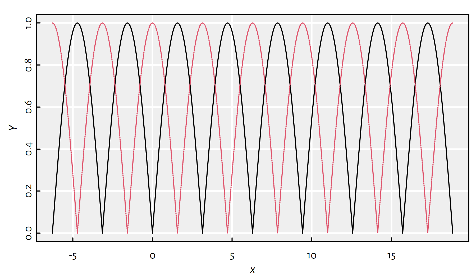

Figure D.1: Example plot with matplot()

D.2.7 Matrix-Vector Operations

Mathematically, there is no generally agreed upon convention defining arithmetic operations between matrices and vectors.

(*) The only exception is the matrix – vector multiplication in the case where an argument is a column or a row vector, i.e., in fact, a matrix. Hence, given \(\mathbf{A}\in\mathbb{R}^{n\times p}\) we may write \(\mathbf{A}\mathbf{x}\) only if \(\mathbf{x}\in\mathbb{R}^{p\times 1}\) is a column vector. Similarly, \(\mathbf{y}\mathbf{A}\) makes only sense whenever \(\mathbf{y}\in\mathbb{R}^{1\times n}\) is a row vector.

Remark.

Please take notice of the fact that we consistently discriminate between different bold math fonts and letter cases: \(\mathbf{X}\) is a matrix, \(\mathbf{x}\) is a row or column vector (still a matrix, but a sequence-like one) and \(\boldsymbol{x}\) is an ordinary vector (one-dimensional sequence).

However, in R, we might sometimes wish to vectorise an arithmetic operation between a matrix and a vector in a row- or column-wise fashion. For example, if \(\mathbf{A}\in\mathbb{R}^{n\times p}\) is a matrix and \(\mathbf{m}\in\mathbb{R}^{1\times p}\) is a row vector, we might want to subtract \(m_i\) from each element in the \(i\)-th column. Here, the apply() function comes in handy again.

Example: to create a centred version of a given matrix, we need to subtract from each element the arithmetic mean of its column.

(A <- cbind(c(1, 2), c(2, 4), c(5, 8)))

##      [,1] [,2] [,3]
## [1,]    1    2    5
## [2,]    2    4    8

(m <- apply(A, 2, mean)) # same as colMeans(A)

## [1] 1.5 3.0 6.5

t(apply(A, 1, function(r) r-m)) # note the transpose here

##      [,1] [,2] [,3]
## [1,] -0.5   -1 -1.5
## [2,]  0.5    1  1.5

The above is equivalent to:

apply(A, 2, function(c) c-mean(c))

##      [,1] [,2] [,3]
## [1,] -0.5   -1 -1.5
## [2,]  0.5    1  1.5

D.3.1 Selecting Individual Elements

Matrices are two-dimensional structures: items are aligned in rows and columns. Hence, to extract an element from a matrix, we will need two indices. Mathematically, given a matrix \(\mathbf{A}\), \(a_{i,j}\) stands for the element in the \(i\)-th row and the \(j\)-th column. The same in R:

A[1, 2] # 1st row, 2nd columns

## [1] 2

B["a", "y"] # using dimnames == B[1,2]

## [1] 2

D.3.2 Selecting Rows and Columns

We will sometimes use the following notation to emphasise that a matrix \(\mathbf{A}\) consists of \(n\) rows or \(p\) columns:

\[ \mathbf{A}=\left[ \begin{array}{c} \mathbf{a}_{1,\cdot} \\ \mathbf{a}_{2,\cdot} \\ \vdots\\ \mathbf{a}_{n,\cdot} \\ \end{array} \right] = \left[ \begin{array}{cccc} \mathbf{a}_{\cdot,1} & \mathbf{a}_{\cdot,2} & \cdots & \mathbf{a}_{\cdot,p} \\ \end{array} \right]. \]

Here, \(\mathbf{a}_{i,\cdot}\) is a row vector of length \(p\), i.e., a \((1\times p)\)-matrix:

\[ \mathbf{a}_{i,\cdot} = \left[ \begin{array}{cccc} a_{i,1} & a_{i,2} & \cdots & a_{i,p} \\ \end{array} \right]. \]

Moreover, \(\mathbf{a}_{\cdot,j}\) is a column vector of length \(n\), i.e., an \((n\times 1)\)-matrix:

\[ \mathbf{a}_{\cdot,j} = \left[ \begin{array}{cccc} a_{1,j} & a_{2,j} & \cdots & a_{n,j} \\ \end{array} \right]^T=\left[ \begin{array}{c} {a}_{1,j} \\ {a}_{2,j} \\ \vdots\\ {a}_{n,j} \\ \end{array} \right], \]

We can extract individual rows and columns from a matrix by using the following notation:

A[1,] # 1st row

## [1] 1 2 3 4

A[,2] # 2nd column

## [1]  2  6 10

B["a",] # of course, B[1,] is still legal

## x y z w 
## 1 2 3 4

B[,"y"]

##  a  b  c 
##  2  6 10

Note that by extracting a single row/column, we get an atomic (one-dimensional) vector. However, we can preserve the dimensionality of the output object by passing drop=FALSE:

A[  1,    , drop=FALSE] # 1st row

##      [,1] [,2] [,3] [,4]
## [1,]    1    2    3    4

A[   ,   2, drop=FALSE] # 2nd column

##      [,1]
## [1,]    2
## [2,]    6
## [3,]   10

B["a",    , drop=FALSE]

##   x y z w
## a 1 2 3 4

B[   , "y", drop=FALSE]

##    y
## a  2
## b  6
## c 10

Now this is what we call proper row and column vectors!

D.3.3 Selecting Submatrices

To create a sub-block of a given matrix we pass two indexers, possibly of length greater than one:

A[1:2, c(1, 2, 4)] # rows 1,2 columns 1,2,4

##      [,1] [,2] [,3]
## [1,]    1    2    4
## [2,]    5    6    8

B[c("a", "b"), c(1, 2, 4)]

##   x y w
## a 1 2 4
## b 5 6 8

A[c(1, 3), 3]

## [1]  3 11

A[c(1, 3), 3, drop=FALSE]

##      [,1]
## [1,]    3
## [2,]   11

D.3.4 Selecting Based on Logical Vectors and Matrices

We can also subset a matrix with a logical matrix of the same size. This always yields a (flat) vector in return.

A[A>8]

## [1]  9 10 11 12

Logical vectors can also be used as indexers:

A[c(TRUE, FALSE, TRUE),] # select 1st and 3rd row

##      [,1] [,2] [,3] [,4]
## [1,]    1    2    3    4
## [2,]    9   10   11   12

A[,colMeans(A)>6] # columns with means > 6

##      [,1] [,2]
## [1,]    3    4
## [2,]    7    8
## [3,]   11   12

B[B[,"x"]>1 & B[,"x"]<=9,] # All rows where x is in (1, 9]

##   x  y  z  w
## b 5  6  7  8
## c 9 10 11 12

D.3.5 Selecting Based on Two-Column Matrices

Lastly, note that we can also index a matrix A with a 2-column matrix I, i.e., A[I]. This allows for an easy access to A[I[1,1], I[1,2]], A[I[2,1], I[2,2]], A[I[3,1], I[3,2]], …

I <- cbind(c(1, 3, 2, 1, 2),
           c(2, 3, 2, 1, 4)
)
A[I]

## [1]  2 11  6  1  8

This is exactly A[1, 2], A[3, 3], A[2, 2], A[1, 1], A[2, 4].

X <- matrix(1:12, byrow=TRUE, nrow=3) # example matrix
dimnames(X)[[2]] <- c("a", "b", "c", "d") # set column names
print(X)
X[1, ]  # selects the 1st row (row with index 1)
X[, 3]  # selects the 3rd column
X[, "a"]  # selects column named "a"
X[1, "a"]  # selects the 1st row and column "a"
X[, c("a", "b", "c")]  # selects 3 columns
X[, -2]  # all but the 2nd column
X[X[,1] > 5, ]  # selects all the rows that have the values in the 1st column greater than 5
X[X[,1]>5, c("a", "b", "c")]  # as above, but return only 3 given columns
X[X[,1]>=5 & X[,1]<=10, ]  # all rows where in the 1st column values are between 5 and 10
X[X[,1]>=5 & X[,1]<=10, c("a", "b", "c")]  # as above, but 3 given columns
X[, c(1, "b", "d")]  # incorrect, atomic vector - 1 will be converted to "1" and there is no column named "1"